The accurate determination of the offset between Mean Sea Level (MSL) and Lowest Astronomical Tide (LAT) is very important for marine and coastal navigation, mapping, and engineering (reduction of bathymetric soundings to LAT, under-keel clearance, and nearshore/offshore infrastructure levelling). The MSL value is obtained from either a local geoid model or from temporary in-situ tide gauge data processed using specialised filters. For many ungauged ports along the Gulf of Guinea, sources like Admiralty Tide Tables (ATT) provide insufficient spatial coverage, necessitating spatial interpolation from regional reference gauges. The low density, heterogeneity, and discontinuity of tide gauge observations impose the use of rigorously evaluated spatial interpolation methods. This study proposes an integrated methodological framework comparing six interpolation techniques: Nearest Neighbour (NN), Inverse-Distance Weighting (IDW), Triangulation (TIN), Spline, Trend Surface, and Kriging. The comparison is based on a regional database of 115 reference ports (106 from the ATT, and nine complementary stations from GLOSS, PSMSL, and UHSLC/JASL networks) spanning 20 West African coastal countries. Three representative Cameroonian test sites are selected: the Rio del Rey Shelf (Betika), the Wouri Estuary (Dibamba-Yassa), and the isolated southern coast (Batanga). The approach combines a unified software implementation, exhaustive comparison and leave-one-out (LOO) cross-validation (MAE, RMSE, bias, R2), convergence analysis and quadratic decomposition of uncertainty components. Results indicate that the optimal interpolation method varies with local reference station density and spatial configuration. At Betika (18 reference stations, 9 retained), IDW yields the best cross validation performance (RMSE ≈ 0.2295 m, R2 ≈ 0.1376) with Kriging close behind. At Dibamba-Yassa (06 stations, 4 retained), Trend Surface performs best (RMSE ≈ 0.1225 m, R2 ≈ 0.2833), followed by Kriging (RMSE=0.1439 m). At Batanga (2 stations only), method comparison fails, illustrating problem degeneration under extreme undersampling. In all cases, interpolation variance σᵢ² accounts for more than 95% of the total error budget, with 95% confidence intervals reaching ±3.6 m to ±4.9 m. The convergence analysis shows that a minimum of 5-7 stations is required to stabilise estimates. The main finding is that network densification is the primary lever for improvement, well ahead of algorithmic optimisation. The study provides validated point estimates for the three sites and a transparent protocol for tidal datum estimation in data sparse coastal regions of the Gulf of Guinea.
| Published in | Journal of Water Resources and Ocean Science (Volume 15, Issue 3) |
| DOI | 10.11648/j.wros.20261503.15 |
| Page(s) | 106-142 |
| Creative Commons |
This is an Open Access article, distributed under the terms of the Creative Commons Attribution 4.0 International License (http://creativecommons.org/licenses/by/4.0/), which permits unrestricted use, distribution and reproduction in any medium or format, provided the original work is properly cited. |
| Copyright |
Copyright © The Author(s), 2026. Published by Science Publishing Group |
Deterministic Method, Geostatistical Method, Hydrography, LOO Cross-validation, MSL-LAT, Spatial Interpolation, Uncertainty, Vertical Reference
No. | Country | Station | (°) | (°) | (m) | 1 |
|---|---|---|---|---|---|---|
Stations from Admiralty Tide Tables | ||||||
1 | Angola | Enseada Cabinda | -5.5500 | 12.2000 | 1.10 | Micro |
2 | Angola | Soyo (Santo Ant.) | -6.1167 | 12.3667 | 1.10 | Micro |
3 | Angola | Porto de Luanda | -8.7500 | 13.2500 | 1.10 | Micro |
4 | Angola | Porto Amboim | -10.7333 | 13.7167 | 1.10 | Micro |
5 | Angola | Porto Lobito | -12.3333 | 13.5667 | 1.10 | Micro |
6 | Angola | Porto de Benguela | -12.5667 | 13.4167 | 0.92 | Micro |
7 | Angola | Baia dos Elefantes | -13.2167 | 12.7333 | 1.10 | Micro |
8 | Angola | Baia de Santa M. | -13.3500 | 12.6500 | 1.10 | Micro |
9 | Angola | Namibe | -15.2000 | 12.1500 | 1.10 | Micro |
10 | Angola | Porto Alexandre | -15.8000 | 11.8500 | 1.10 | Micro |
11 | Angola | Baia dos Tigres | -16.6000 | 11.8167 | 1.10 | Micro |
12 | Atlantic Is. | Ascension Island | -7.9167 | -14.0333 | 0.70 | Micro |
13 | Atlantic Is. | Saint Helena Is. | -15.9167 | -5.7000 | 0.50 | Micro |
14 | Benin | Cotonou | 6.3473 | 2.4105 | 0.93 | Micro |
15 | Cameroon | Rio Del Rey Ent. | 4.5000 | 8.8500 | 1.41 | Micro |
16 | Cameroon | Man O War Bay | 3.9667 | 9.3670 | 1.20 | Micro |
17 | Cameroon | Entrance Bimbia | 4.0667 | 9.1170 | 1.10 | Micro |
18 | Cameroon | Tiko-Bimbia R. | 4.0500 | 9.2170 | 1.20 | Micro |
19 | Cameroon | Cap Cameroun | 3.9000 | 9.4500 | 1.40 | Micro |
20 | Cameroon | Douala | 4.0333 | 9.7000 | 1.62 | Micro |
21 | Cameroon | Manoka | 3.9167 | 9.6000 | 1.42 | Micro |
22 | Cameroon | Malimba | 3.5333 | 9.3833 | 1.32 | Micro |
23 | Cameroon | Kribi | 2.9167 | 9.9333 | 1.00 | Micro |
24 | Congo | Pointe Noire | -4.7886 | 11.8329 | 0.96 | Micro |
25 | DR Congo | Bulabemba | -6.0500 | 12.4500 | 1.00 | Micro |
26 | Eq. Guinea | Pagalu (Annobon) | -1.4167 | 5.6333 | 0.80 | Micro |
27 | Eq. Guinea | Bata | 1.8667 | 9.7667 | 1.02 | Micro |
28 | Eq. Guinea | Rio Benito | 1.5667 | 9.6333 | 0.96 | Micro |
29 | Eq. Guinea | Cogo-Rio Muni | 1.0833 | 9.7000 | 1.49 | Micro |
30 | Eq. Guinea | Malabo | 3.7500 | 8.7833 | 1.16 | Micro |
31 | Eq. Guinea | Bahia de Luba | 3.2833 | 8.5833 | 1.02 | Micro |
32 | Gabon | Libreville | 0.3833 | 9.4500 | 1.29 | Micro |
33 | Gabon | Pointe Owendo | 0.2886 | 9.5101 | 1.45 | Micro |
34 | Gabon | Port Gentil | -0.7149 | 8.7852 | 1.45 | Micro |
35 | Gabon | Cap Esterias | 0.6167 | 9.5000 | 1.40 | Micro |
36 | Gabon | Cap Lopez | -0.6827 | 8.8580 | 1.23 | Micro |
37 | Ghana | Takoradi | 4.8869 | -1.7401 | 0.76 | Micro |
38 | Ghana | Sekondi | 4.9534 | -1.7369 | 0.98 | Micro |
39 | Ghana | Accra | 5.5599 | -0.1964 | 0.98 | Micro |
40 | Ghana | Tema | 5.6579 | 0.0260 | 0.88 | Micro |
41 | Guinea-Conakry | Rio Nunez App. | 10.6638 | -14.5844 | 2.65 | Meso |
42 | Guinea-Conakry | Port Kamsar | 10.6638 | -14.5845 | 3.03 | Meso |
43 | Guinea-Conakry | Conakry | 9.5102 | -13.7158 | 2.07 | Meso |
44 | Guinea-Bissau | Varela | 12.2865 | -16.5949 | 1.33 | Micro |
45 | Guinea-Bissau | Cacheu | 12.2746 | -16.1632 | 1.60 | Micro |
46 | Guinea-Bissau | Ilheu de Caio | 12.2794 | -16.1655 | 1.90 | Micro |
47 | Guinea-Bissau | Ponta Biombo | 11.7407 | -15.9516 | 2.33 | Meso |
48 | Guinea-Bissau | Bissau | 11.8600 | -15.5767 | 2.89 | Meso |
49 | Guinea-Bissau | Jabada | 11.9467 | -15.3477 | 3.34 | Meso |
50 | Guinea-Bissau | Porto Gole | 11.9668 | -15.1347 | 3.95 | Meso |
51 | Guinea-Bissau | Bolama | 11.5772 | -15.4798 | 2.88 | Meso |
52 | Guinea-Bissau | Sanincha | 11.8599 | -15.5767 | 2.90 | Meso |
53 | Guinea-Bissau | Bubaque | 11.3000 | -15.8272 | 2.54 | Meso |
54 | Guinea-Bissau | João Vieira | 11.1333 | -15.6318 | 2.59 | Meso |
55 | Guinea-Bissau | Cacine | 11.1318 | -15.0233 | 3.31 | Meso |
56 | Ivory Coast | Abidjan Entrance | 5.3327 | -4.0296 | 0.74 | Micro |
57 | Liberia | Monrovia | 6.3440 | -10.7930 | 0.90 | Micro |
58 | Liberia | Balfu Bay | 5.1529 | -9.2901 | 0.73 | Micro |
59 | Liberia | Sinoe Bay | 5.2901 | -8.8153 | 0.91 | Micro |
60 | Namibia | Walvis Bay | -22.9500 | 14.4833 | 0.98 | Micro |
61 | Namibia | Luderitz | -26.3167 | 15.0167 | 0.94 | Micro |
62 | Nigeria | Warri | 5.5499 | 5.7671 | 1.04 | Micro |
63 | Nigeria | Forcados River | 5.3700 | 5.4399 | 0.97 | Micro |
64 | Nigeria | Opobo River | 4.5147 | 7.5284 | 1.10 | Micro |
65 | Nigeria | Kwa Ibo River | 4.6660 | 7.9884 | 1.13 | Micro |
66 | Nigeria | Bonny Town | 4.4383 | 7.1592 | 1.48 | Micro |
67 | Nigeria | Bonny River Bar | 4.4296 | 7.1956 | 1.43 | Micro |
68 | Nigeria | No 2 Buoy | 4.3833 | 8.4000 | 1.10 | Micro |
69 | Nigeria | Bakassi Bank | 4.4500 | 8.4000 | 1.22 | Micro |
70 | Nigeria | Jamestown | 4.4833 | 8.1170 | 1.48 | Micro |
71 | Nigeria | James Island | 4.8667 | 8.1170 | 1.34 | Micro |
72 | Nigeria | Calabar | 4.9667 | 8.3170 | 2.09 | Meso |
73 | Nigeria | Inikoi Island | 4.8500 | 8.3833 | 1.60 | Micro |
74 | Nigeria | Lagos Bar | 6.5255 | 3.3785 | 0.78 | Micro |
75 | Nigeria | Badagry Creek | 6.4244 | 3.2440 | 0.61 | Micro |
76 | Nigeria | Jamestown (2) | 5.0167 | 8.3833 | 1.48 | Micro |
77 | Nigeria | James Island (2) | 5.5187 | 5.7498 | 1.54 | Micro |
78 | Nigeria | Ogidigbe | 5.5558 | 5.1822 | 0.97 | Micro |
79 | Nigeria | Forcados | 5.3456 | 5.3463 | 0.82 | Micro |
80 | Nigeria | Akassa | 4.3222 | 6.0625 | 0.98 | Micro |
81 | Nigeria | Bonny River | 4.4769 | 7.1744 | 1.48 | Micro |
82 | Nigeria | Ford Point | 4.8027 | 7.0018 | 1.52 | Micro |
83 | Nigeria | Port Harcourt | 4.8478 | 6.9650 | 1.46 | Micro |
84 | Nigeria | Sapele | 5.8964 | 5.6715 | 0.91 | Micro |
85 | Nigeria | Apapa | 6.4574 | 3.3644 | 0.88 | Micro |
86 | Nigeria | Youngtown | 4.4544 | 6.9905 | 0.59 | Micro |
87 | Nigeria | Koko | 5.9993 | 5.4460 | 0.56 | Micro |
88 | Nigeria | Madagho | 5.6019 | 5.2301 | 0.86 | Micro |
89 | Nigeria | Rugged Point | 5.5827 | 5.3727 | 0.75 | Micro |
90 | Sao Tome & Pr. | Ilha do Principe | 1.6000 | 7.2500 | 1.20 | Micro |
91 | Sao Tome & Pr. | Ilha do Sao Tome | 0.2167 | 6.7500 | 1.20 | Micro |
92 | Sierra Leone | Freetown | 8.4844 | -13.2344 | 1.77 | Micro |
93 | Sierra Leone | Shenge Point | 7.9007 | -12.9408 | 1.65 | Micro |
94 | Sierra Leone | Sheather Rock | 7.7513 | -12.7971 | 1.68 | Micro |
95 | Sierra Leone | Bonthe | 7.5312 | -12.5014 | 0.92 | Micro |
96 | South Africa | Port Nolloth | -29.2500 | 16.0833 | 1.09 | Micro |
97 | South Africa | Lamberts Bay | -32.0833 | 18.3333 | 0.85 | Micro |
98 | South Africa | Saint Helena Bay | -32.7333 | 17.8333 | 0.90 | Micro |
99 | South Africa | Saldanha | -33.0323 | 17.9214 | 0.99 | Micro |
100 | South Africa | Schrywershoek | -33.0615 | 18.0419 | 0.98 | Micro |
101 | South Africa | Cape Town | -33.9242 | 18.4127 | 0.98 | Micro |
102 | South Africa | Simons Town | -34.1929 | 18.4379 | 1.00 | Micro |
103 | South Africa | Hermanus | -34.4166 | 19.2453 | 1.02 | Micro |
104 | South Africa | Mossel Bay | -34.1837 | 22.1267 | 1.17 | Micro |
105 | South Africa | Knysna | -34.0309 | 23.0226 | 1.06 | Micro |
106 | Togo | Lome | 6.1284 | 1.2213 | 1.15 | Micro |
Complementary Stations - GLOSS / PSMSL / UHSLC2 - ATT2 | ||||||
107 | Senegal | Dakar | 14.6333 | -17.4500 | 0.82 | Micro |
108 | Mauritania | Nouakchott | 18.0830 | -15.9800 | 0.97 | Micro |
109 | Mauritania | Nouadhibou (Port-Etienne) | 20.9000 | -17.0500 | 1.00 | Micro |
110 | Gambia | Banjul | 13.4500 | -16.5700 | 1.05 | Micro |
111 | Ivory Coast | Abidjan (GLOSS) | 5.2500 | -4.2500 | 0.74 | Micro |
112 | Cameroon | Port Sonara (Limbe) | 4.0050 | 9.1250 | 1.20 | Micro |
113 | Congo | Pointe Noire (GLOSS) | -4.7830 | 11.8330 | 0.96 | Micro |
114 | Sao Tome & Pr. | Sao Tome (PSMSL) | 0.0167 | 6.5167 | 1.20 | Micro |
115 | Cape Verde | Palmeira (Sal) | 16.7550 | -22.9300 | 0.65 | Micro |
Parameter | Dibamba-Yassa | Betika | Batanga |
|---|---|---|---|
Geographic Coord. (WGS84) | Lat=03°56'26" N | Lat=04°16'27" N | Lat=02°48'48" N |
Lon=009°49'14" E | Lon=008°23'07" E | Lon=009°49'00" E | |
Water Depth (LAT) | 5.0 m | 21.5 m | 30.0 m |
Model | Variogram formula |
|---|---|
Spherical |
|
Exponential |
|
Gaussian |
|
Matern 3/2 |
|
Matern 5/2 |
|
Metric | Formula | Interpretation |
|---|---|---|
MAE |
| Mean Absolute Error: mean absolute deviation between observed and estimated values. |
RMSE |
| Root Mean Square Error: strongly penalises large and outlying errors. |
R² |
| Coefficient of Determination: proportion of variance explained (Z̄=mean of observations). |
Bias |
| Systematic Bias: tendency to consistently under- or over-estimate values. |
Parameter | Value |
|---|---|
Available stations (100 km radius) | 18 |
Retained stations (CV | 9 |
Inter-station distances (km) | 12.2 - 133.0 (mean ≈ 78.3) |
Spatial extent (lat × lon) | ≈ 1.73° × 2.25° |
Spatial variance σ² (m²) | 0.0611 (σ ≈ 0.25 m; CV=18.8%) |
Station density / 1,000 km² | 0.347 |
Mean MSL-LAT of 18 stations (m) | 1.31 |
MSL-LAT range (m) | 1.02 (Bahia de Luba) - 2.09 (Calabar) |
Rank | Method | Score | σₜ (m) | Level |
|---|---|---|---|---|
1 | IDW | 0.370 | ±2.479 | AccepTable |
2 | Kriging | 0.358 | ±2.479 | AccepTable |
3 | TIN | 0.219 | ±2.483 | Limited |
4 | Trend | 0.069 | ±2.488 | Limited |
5 | NN | -0.125 | ±2.493 | Limited |
6 | Spline | -0.149 | ±2.494 | Limited |
Method | NN | IDW | TIN | Trend | Spline | Kriging |
|---|---|---|---|---|---|---|
NN | 1.000 | 0.893 | 0.896 | 0.722 | 0.923 | 0.712 |
IDW | 0.893 | 1.000 | 0.768 | 0.837 | 0.890 | 0.785 |
TIN | 0.896 | 0.768 | 1.000 | 0.692 | 0.815 | 0.721 |
Trend | 0.722 | 0.837 | 0.692 | 1.000 | 0.845 | 0.597 |
Spline | 0.923 | 0.890 | 0.815 | 0.845 | 1.000 | 0.640 |
Kriging | 0.712 | 0.785 | 0.721 | 0.597 | 0.640 | 1.000 |
Component | Value (m²) | Share in σt² (%) |
|---|---|---|
σᵢ² (interpolation variance, spatial configure) | 6.0827 | ≈ 96% |
σd² (data source quality -IDW) | 0.0527 | ≈ 1% |
σd² (data source quality -NN) | 0.1225 | (reference) |
σm² (model specification -all methods) | 0.0098 | < 1% |
σt (IDW) | ±2.479 m | - |
CI₉₅ (IDW) | ±4.859 m | - |
Parameter | Value |
|---|---|
Available stations (68 km radius) | 6 |
Minimum inter-station distance (km) | 11.8 |
Maximum inter-station distance (km) | 65.8 |
Mean inter-station distance (km) | 37.0 |
Spatial extent (lat × lon) | ≈ 0.52° × 0.48° |
Spatial variance σ² (m²) | 0.0209 (σ ≈ 0.145 m; CV=10.6%) |
Station density / 1,000 km² | 1.766 |
Mean MSL-LAT of 6 stations (m) | 1.36 |
MSL-LAT range (m) | 1.20 (Tiko-Bimbia River) - 1.62 (Douala) |
Rank | Method | Score | σₜ (m) | Level |
|---|---|---|---|---|
1 | Trend | 0.539 | ±2.117 | Good |
2 | Kriging | 0.431 | ±2.118 | AccepTable |
3 | NN | 0.423 | ±2.119 | AccepTable |
4 | TIN | 0.352 | ±2.119 | AccepTable |
5 | Spline | 0.245 | ±2.121 | Limited |
6 | IDW | 0.224 | ±2.121 | Limited |
Method | NN | IDW | TIN | Trend | Spline | Kriging |
|---|---|---|---|---|---|---|
NN | 1.000 | 0.624 | 0.512 | 0.830 | 0.780 | 0.654 |
IDW | 0.624 | 1.000 | 0.959 | 0.695 | 0.681 | 0.972 |
TIN | 0.512 | 0.959 | 1.000 | 0.709 | 0.701 | 0.978 |
Trend | 0.830 | 0.695 | 0.709 | 1.000 | 0.988 | 0.813 |
Spline | 0.780 | 0.681 | 0.701 | 0.988 | 1.000 | 0.810 |
Kriging | 0.654 | 0.972 | 0.978 | 0.813 | 0.810 | 1.000 |
Component | Value (m²) | Share in σₜ² (%) |
|---|---|---|
σᵢ² (interpolation variance, spatial configure) | 4.4610 | > 95% |
σd² (data quality - Trend Surface) | 0.0150 | ≈ 1% |
σd² (data quality - NN) | 0.0211 | (reference) |
σm² (model specification - all methods) | 0.0058 | < 1% |
σₜ (Trend Surface, 6 stations) | ±2.117 m | - |
CI₉₅ (Trend Surface, 6 stations) | ±4.149 m | - |
σₜ (Trend Surface, dedicated validation - 4 stations) | ±1.834 m | - |
CI₉₅ (Trend Surface, dedicated validation) | ±3.595 m | - |
Parameter | Value |
|---|---|
Number of available stations | 2 (Kribi and Malimba) |
Distances to site (km) | 17.3 (Kribi, south); 93.4 (Malimba, north) |
Mean distance to site (km) | 55.4 |
Spatial extent (lat × lon) | ≈ 0.62° × 0.55° |
MSL-LAT of stations (m) | 1.00 (Kribi); 1.32 (Malimba) |
Spatial variance σ² (m²) | ≈ 0.0256 (n=2, statistically non-significant) |
Station density / 1,000 km² | ≈ 0.302 |
Coefficient of variation CV (%) | 13.8 (uninterpreTable with n=2) |
Rank | Method | Score | σₜ (m) | Level |
|---|---|---|---|---|
1-6 | All methods | -0.716 | ±2.375 | Unusable |
Component | Value (m²) | Share in σₜ² (%) |
|---|---|---|
σᵢ² (interpolation variance) | 5.5826 | > 98% |
σd² (data source quality -NN) | 0.1447 | ≈ 2% |
σm² (model specification) | 0.0032 | < 0.1% |
σₜ | ±2.375 m | - |
CI₉₅ | ±4.662 m | - |
Parameter | Dibamba-Yassa | Betika | Batanga |
|---|---|---|---|
Context | Wouri Estuary (<20 m) | Rio del Rey Shelf (20-50 m) | Isolated open coast |
Available / retained stations | 6 / 4 | 18 / 9 | 2 / 2 |
Distance range (km) | 16.9 - 50.4 | 12.2 - 133.0 | 17.3 - 93.4 |
Spatial extent (lat × lon) | ≈ 0.52° × 0.48° | ≈ 1.73° × 2.25° | ≈ 0.62° × 0.55° |
Density (st./1,000 km²) | 1.766 | 0.347 | 0.302 |
Spatial σ (m) / CV (%) | 0.145 / 10.6 | 0.25 / 18.8 | 0.16 / 13.8 (n.s.) |
Retained method | Trend Surface (kopt=4) | IDW (kopt=9) | NN (default, kopt=1)) |
MSL-LAT offset (m) | 1.571 | 1.147 | 1.00 |
Best RMSE (m) | 0.1225 (Trend) | 0.2295 (IDW) | 0.320 (all) |
Best R² | 0.2833 (Trend) | 0.1376 (IDW) | -3.000 (all) |
σₜ / CI₉₅ (m) | ±1.834 / ±3.595 | ±2.479 / ±4.859 | ±2.375 / ±4.662 |
Performance level | Good | AccepTable (moderate) | Unusable |
Relative confidence (0-3) | 2 | 1-2 | 0 |
Rank | Dibamba-Yassa (RMSE, m) | Betika (RMSE, m) | Batanga (RMSE, m) |
|---|---|---|---|
1 | Trend (0.1225) | IDW (0.2295) | All (0.320) |
2 | Kriging (0.1439) | Kriging (0.2343) | - |
3 | NN (0.1454) | TIN (0.2706) | - |
4 | TIN (0.1571) | Trend (0.3095) | - |
5 | Spline (0.1746) | NN (0.3501) | - |
6 | IDW (0.1777) | Spline (0.3562) | - |
RMSE range | 0.1225 - 0.1777 (0.055 m) | 0.2295 - 0.3562 (0.127 m) | 0 (degeneration) |
Site | σᵢ² (m²) | σd² (m²) | σm² (m²) | σₜ (m) | Share σᵢ² (%) |
|---|---|---|---|---|---|
Dibamba-Yassa (4 st.) | 4.4610 | 0.015 - 0.032 | 0.006 | ±1.834 | > 95% |
Betika (9 st.) | 6.0827 | 0.053 - 0.123 | 0.010 | ±2.479 | ≈ 96% |
Batanga (2 st.) | 5.5826 | 0.145 | 0.003 | ±2.375 | > 98% |
Site | Context | Reliability | Operational Recommendation |
|---|---|---|---|
Dibamba-Yassa | Complex estuary (<20 m) | Good | Trend Surface suitable for operational use. In-situ validation by temporary tide gauge (≥15 days) recommended for critical applications. |
Betika | Shelf (20-50 m) | Moderate to accepTable | Offshore surveys with conservative vertical margin ≈ ±4.9 m. Densify network to south of site. |
Batanga | Isolated open coast | None | Use discouraged without dedicated tide gauge campaign. Nearest station value for indicative use only. |
Density / Context | Preferred Method | kopt | Typical RMSE | Operational CI₉₅ |
|---|---|---|---|---|
≥5-7 stations, extent >1° (Betika, Nigeria/Cameroon clusters) | 1-IDW, 2-Kriging, 3-TIN | 6-10 | 0.22-0.29 m | ±4.9 m; conservative margins |
2-6 stations, extent <0.7° (Dibamba-Yassa, estuaries) | 1-Trend, 2-Kriging, 3-NN | 2-4 | 0.12-0.15 m | ±3.6 m; in-situ validation required |
<3 stations, isolated coast (Batanga, Angola, Guinea) | NN (nearest station) | 1 | 0.32 m | Invalidate; tide gauge campaign required |
ATT | Admiralty Tide Tables |
BLUE | Best Linear Unbiased Estimator |
CI | Confidence Interval |
GCV | Generalised Cross-Validation |
GLOSS | Global Sea Level Observing System |
IDW | Inverse-Distance Weighting |
IHO | International Hydrographic Organization |
JASL | Joint Archive for Sea Level |
LAT | Lowest Astronomical Tide |
LOO | Leave-One-Out |
LOOCV | Leave-One-Out Cross-Validation |
MAE | Mean Absolute Error |
MSL | Mean Sea Level |
NN | Nearest Neighbour |
PSMSL | Permanent Service for Mean Sea Level |
RMSE | Root Mean Square Error |
TCARI | Tidal Constituent and Residual Interpolation |
TIN | Triangulated Irregular Network |
TPS | Thin-Plate Spline |
UHSLC | University of Hawaii Sea Level Center |
UTM | Universal Transverse Mercator |
WGS84 | World Geodetic System 1984 |
| [1] |
International Hydrographic Organization. Manual on Hydrography (C-13). Monaco: IHO; 2020. Available from:
https://iho.int/uploads/user/pubs/cb/c-13/c-13_ed3-0-0_2020_EN.pdf |
| [2] | Pugh, D., Woodworth, P. Sea-Level Science: Understanding Tides, Surges, Tsunamis and Mean Sea-Level Changes. Cambridge: Cambridge University Press; 2014. |
| [3] | Slobbe, D. C., Sumihar, J., Frederikse, T., Verlaan, M., Klees, R., Zijl, F., Farahani, H. H., Broekman, R. A Kalman filter approach to realize the lowest astronomical tide surface. Marine Geodesy. 2018, 41(1), 44-67. |
| [4] | Erol, B., Erol, S., Çelik, R. N. Height transformation using regional geoids and GPS/levelling in Turkey. Survey Review. 2008, 40(307), 2-18. |
| [5] | Mfeze, M. Harmonic Modeling of Tidal Fluctuations in the Wouri Estuary: A Unified Analysis for Accurate Tide Prediction at the Port Authority of Douala. Journal of Geosciences and Geomatics. 2025, 13(1), 1-22. |
| [6] |
United Kingdom Hydrographic Office. Admiralty Tide Tables, Vol. 8: South East Atlantic Ocean, West Africa and Mediterranean (NP208-23). Taunton, UK: UKHO; 2026. Available from:
https://www.admiralty.co.uk/publications/publications/admiralty-tide-Tables |
| [7] | Wöppelmann, G., Marcos, M. Vertical land motion as a key to understanding sea level change and variability. Reviews of Geophysics. 2016, 54(1), 64-92. |
| [8] | Intergovernmental Oceanographic Commission (IOC/UNESCO). Global Sea Level Observing System (GLOSS) Implementation Plan 2022. Paris: IOC/UNESCO; 2022. Available from: |
| [9] | Woodworth, P. L., Hunter, J. R., Marcos, M., Caldwell, P., Menendez, M., Haigh, I. D. Towards a global higher-frequency sea level dataset. Geoscience Data Journal. 2017, 3, 50-59. |
| [10] | Intergovernmental Oceanographic Commission. Manual on Sea Level Measurement and Interpretation, Volume V: Radar Gauges. Paris: IOC/UNESCO; 2017. Available from: |
| [11] | Almar, R., et al. Coastal Zone Changes in West Africa: Challenges and Opportunities for Satellite Earth Observations. Surveys in Geophysics. 2022, 43(1), 249-275. |
| [12] | Lloyd, C. D. Local Models for Spatial Analysis, 2nd ed. Boca Raton, FL: CRC Press; 2010. |
| [13] | Chilès, J. P., Delfiner, P. Geostatistics: Modeling Spatial Uncertainty, 2nd ed. Hoboken, NJ: Wiley; 2012. |
| [14] | Turner, J. F., Iliffe, J. C., Ziebart, M. K., Wilson, C., Horsburgh, K. J. Interpolation of tidal levels in the coastal zone for the creation of a hydrographic datum. Journal of Atmospheric and Oceanic Technology. 2010, 27(3), 605-613. |
| [15] | Orton, P., Georgas, S., Blumberg, A., Pullen, J. Detailed modeling of recent severe storm tides in estuaries of the New York City region. Journal of Geophysical Research: Oceans. 2012, 117, C09030. |
| [16] |
International Hydrographic Organization. IHO Standards for Hydrographic Surveys: Supplementary Guidance (M-3). Monaco: IHO; 2022. Available from:
https://iho.int/uploads/user/pubs/standards/m-3/M-3-Ed2-2.0.0-EN.pdf |
| [17] | Robin, C., Nudds, S., MacAulay, P., Godin, A., De Lange Boom, B., Bartlett, J. Hydrographic vertical separation surfaces (HyVSEPs) for the tidal waters of Canada. Marine Geodesy. 2016, 39(2), 195-222. |
| [18] | Iliffe, J. C., Turner, J. F., Ziebart, M. K., Talbot, A. J. Ellipsoidal and chart datums in hydrographic surveying: Defining the vertical uncertainty budget. Journal of Navigation. 2013, 66(2), 205-220. |
| [19] | Li, J., Heap, A. D. Spatial interpolation methods applied in the environmental sciences: A review. Environmental Modelling & Software. 2014, 53, 173-189. |
| [20] | Matheron, G. Principles of geostatistics. Economic Geology. 1963, 58(8), 1246-1266. |
| [21] | Guo, J., Hwang, C., Chang, X., Liu, Y. Improved inversion of tide gauge positions from satellite altimetry. Geophysical Research Letters. 2021, 48(5), e2020GL091997. |
| [22] | Kemgang Ghomsi, F. E., et al. Sea level variability in Gulf of Guinea from satellite altimetry. Scientific Reports. 2024, 14(1), 5061. |
| [23] |
African Union Commission. Programme for Africa’s Coastal Transformation: Framework for Action (PACT). Addis Ababa: African Union; 2023. Available from:
https://au.int/en/documents/20230612/programme-africas-coastal-transformation-framework-action |
| [24] | L. Djeumeni Noubissie, "Sea level variations in the Gulf of Guinea and coastal risks: focus on the Wouri estuary" (in French), Ph.D. dissertation, Université Toulouse III - Paul Sabatier & Université de Douala, 2024. |
| [25] | Idier, D., Castelle, B., Lambert, J., Marieu, V., Pedreros, R. C., Silva, D. A. F. Wave climate and coastal processes along the West African coast. Continental Shelf Research. 2018, 167, 45-60. |
| [26] | Reverdin, G., McPhaden, M. J. Seasonal upwelling influence on Gulf of Guinea hydrodynamics. Journal of Physical Oceanography. 2021, 51(6), 1457-1475. |
| [27] | Holgate, S. J., et al. New data systems and products at the Permanent Service for Mean Sea Level. Journal of Coastal Research. 2013, 29(3), 493-504. |
| [28] | Wöppelmann, G., et al. Dakar sea-level records: 200 years of tide gauge data for sea-level research. SONEL/PSMSL Technical Report; 2008. |
| [29] | Sarr, C. A. T., Ndour, M. M. M., Haddad, M., Sakho, I. Estimation of sea level rise on the West African Coasts: Case of Senegal, Mauritania and Cape Verde. International Journal of Geosciences. 2021, 12(2), 121-137. |
| [30] | Arnould, O., Testut, C. E., Picot, N. Coastal altimetry for tidal analysis in the Gulf of Guinea. Journal of Geophysical Research: Oceans. 2020, 125(8), e2020JC016234. |
| [31] | Sinnott, R. W. Virtues of the haversine. Sky & Telescope. 1984, 68(2), 158-159. |
| [32] | Vincenty, T. Direct and inverse solutions of geodesics on the ellipsoid with application of nested equations. Survey Review. 1975, 23(176), 88-93. |
| [33] | Arlot, S., Celisse, A. A survey of cross-validation procedures for model selection. Statistics Surveys. 2010, 4, 40-79. |
| [34] | Stone, M. Cross-validatory choice and assessment of statistical predictions. Journal of the Royal Statistical Society: Series B (Methodological). 1974, 36(2), 111-133. |
| [35] | Shepard, D. A two-dimensional interpolation function for irregularly-spaced data. In Proceedings of the 1968 ACM National Conference, New York, USA, 1968; pp. 517-524. |
| [36] | Bowyer, A. Computing Dirichlet tessellations. The Computer Journal. 1981, 24(2), 162-166. |
| [37] | Watson, D. F. Computing the n-dimensional Delaunay tessellation with application to Voronoi polytopes. The Computer Journal. 1981, 24(2), 167-172. |
| [38] | Wahba, G. Spline Models for Observational Data. Philadelphia, PA: Society for Industrial and Applied Mathematics (SIAM); 1990. |
| [39] | Craven, P., Wahba, G. Smoothing noisy data with spline functions: Estimating the correct degree of smoothing by the method of generalized cross-validation. Numerische Mathematik. 1979, 31(4), 377-403. |
| [40] | Krige, D. G. A statistical approach to some mine valuation and allied problems on the Witwatersrand. Journal of the Chemical, Metallurgical and Mining Society of South Africa. 1951, 52, 119-139. |
| [41] | Hess, K., Schmalz, R., Zervas, C., Collier, W. Tidal Constituent And Residual Interpolation (TCARI): A New Method for the Tidal Correction of Bathymetric Data. NOAA Technical Report NOS CS 4; 2004. Available from: |
APA Style
Mfeze, M. (2026). Spatial Interpolation of Hydrographic Vertical References in the Gulf of Guinea: Hierarchical Ranking of Geostatistical and Deterministic Methods by LOO Cross-validation. Journal of Water Resources and Ocean Science, 15(3), 106-142. https://doi.org/10.11648/j.wros.20261503.15
ACS Style
Mfeze, M. Spatial Interpolation of Hydrographic Vertical References in the Gulf of Guinea: Hierarchical Ranking of Geostatistical and Deterministic Methods by LOO Cross-validation. J. Water Resour. Ocean Sci. 2026, 15(3), 106-142. doi: 10.11648/j.wros.20261503.15
@article{10.11648/j.wros.20261503.15,
  author = {Michel Mfeze},
  title = {Spatial Interpolation of Hydrographic Vertical References in the Gulf of Guinea: Hierarchical Ranking of Geostatistical and Deterministic Methods by LOO Cross-validation},
  journal = {Journal of Water Resources and Ocean Science},
  volume = {15},
  number = {3},
  pages = {106-142},
  doi = {10.11648/j.wros.20261503.15},
  url = {https://doi.org/10.11648/j.wros.20261503.15},
  eprint = {https://article.sciencepublishinggroup.com/pdf/10.11648.j.wros.20261503.15},
  abstract = {The accurate determination of the offset between Mean Sea Level (MSL) and Lowest Astronomical Tide (LAT) is very important for marine and coastal navigation, mapping, and engineering (reduction of bathymetric soundings to LAT, under-keel clearance, and nearshore/offshore infrastructure levelling). The MSL value is obtained from either a local geoid model or from temporary in-situ tide gauge data processed using specialised filters. For many ungauged ports along the Gulf of Guinea, sources like Admiralty Tide Tables (ATT) provide insufficient spatial coverage, necessitating spatial interpolation from regional reference gauges. The low density, heterogeneity, and discontinuity of tide gauge observations impose the use of rigorously evaluated spatial interpolation methods. This study proposes an integrated methodological framework comparing six interpolation techniques: Nearest Neighbour (NN), Inverse-Distance Weighting (IDW), Triangulation (TIN), Spline, Trend Surface, and Kriging. The comparison is based on a regional database of 115 reference ports (106 from the ATT, and nine complementary stations from GLOSS, PSMSL, and UHSLC/JASL networks) spanning 20 West African coastal countries. Three representative Cameroonian test sites are selected: the Rio del Rey Shelf (Betika), the Wouri Estuary (Dibamba-Yassa), and the isolated southern coast (Batanga). The approach combines a unified software implementation, exhaustive comparison and leave-one-out (LOO) cross-validation (MAE, RMSE, bias, R2), convergence analysis and quadratic decomposition of uncertainty components. Results indicate that the optimal interpolation method varies with local reference station density and spatial configuration. At Betika (18 reference stations, 9 retained), IDW yields the best cross validation performance (RMSE ≈ 0.2295 m, R2 ≈ 0.1376) with Kriging close behind. At Dibamba-Yassa (06 stations, 4 retained), Trend Surface performs best (RMSE ≈ 0.1225 m, R2 ≈ 0.2833), followed by Kriging (RMSE=0.1439 m). At Batanga (2 stations only), method comparison fails, illustrating problem degeneration under extreme undersampling. In all cases, interpolation variance σᵢ² accounts for more than 95% of the total error budget, with 95% confidence intervals reaching ±3.6 m to ±4.9 m. The convergence analysis shows that a minimum of 5-7 stations is required to stabilise estimates. The main finding is that network densification is the primary lever for improvement, well ahead of algorithmic optimisation. The study provides validated point estimates for the three sites and a transparent protocol for tidal datum estimation in data sparse coastal regions of the Gulf of Guinea.},
 year = {2026}
}
TY  - JOUR
T1  - Spatial Interpolation of Hydrographic Vertical References in the Gulf of Guinea: Hierarchical Ranking of Geostatistical and Deterministic Methods by LOO Cross-validation
AU  - Michel Mfeze
Y1  - 2026/06/30
PY  - 2026
N1  - https://doi.org/10.11648/j.wros.20261503.15
DO  - 10.11648/j.wros.20261503.15
T2  - Journal of Water Resources and Ocean Science
JF  - Journal of Water Resources and Ocean Science
JO  - Journal of Water Resources and Ocean Science
SP  - 106
EP  - 142
PB  - Science Publishing Group
SN  - 2328-7993
UR  - https://doi.org/10.11648/j.wros.20261503.15
AB  - The accurate determination of the offset between Mean Sea Level (MSL) and Lowest Astronomical Tide (LAT) is very important for marine and coastal navigation, mapping, and engineering (reduction of bathymetric soundings to LAT, under-keel clearance, and nearshore/offshore infrastructure levelling). The MSL value is obtained from either a local geoid model or from temporary in-situ tide gauge data processed using specialised filters. For many ungauged ports along the Gulf of Guinea, sources like Admiralty Tide Tables (ATT) provide insufficient spatial coverage, necessitating spatial interpolation from regional reference gauges. The low density, heterogeneity, and discontinuity of tide gauge observations impose the use of rigorously evaluated spatial interpolation methods. This study proposes an integrated methodological framework comparing six interpolation techniques: Nearest Neighbour (NN), Inverse-Distance Weighting (IDW), Triangulation (TIN), Spline, Trend Surface, and Kriging. The comparison is based on a regional database of 115 reference ports (106 from the ATT, and nine complementary stations from GLOSS, PSMSL, and UHSLC/JASL networks) spanning 20 West African coastal countries. Three representative Cameroonian test sites are selected: the Rio del Rey Shelf (Betika), the Wouri Estuary (Dibamba-Yassa), and the isolated southern coast (Batanga). The approach combines a unified software implementation, exhaustive comparison and leave-one-out (LOO) cross-validation (MAE, RMSE, bias, R2), convergence analysis and quadratic decomposition of uncertainty components. Results indicate that the optimal interpolation method varies with local reference station density and spatial configuration. At Betika (18 reference stations, 9 retained), IDW yields the best cross validation performance (RMSE ≈ 0.2295 m, R2 ≈ 0.1376) with Kriging close behind. At Dibamba-Yassa (06 stations, 4 retained), Trend Surface performs best (RMSE ≈ 0.1225 m, R2 ≈ 0.2833), followed by Kriging (RMSE=0.1439 m). At Batanga (2 stations only), method comparison fails, illustrating problem degeneration under extreme undersampling. In all cases, interpolation variance σᵢ² accounts for more than 95% of the total error budget, with 95% confidence intervals reaching ±3.6 m to ±4.9 m. The convergence analysis shows that a minimum of 5-7 stations is required to stabilise estimates. The main finding is that network densification is the primary lever for improvement, well ahead of algorithmic optimisation. The study provides validated point estimates for the three sites and a transparent protocol for tidal datum estimation in data sparse coastal regions of the Gulf of Guinea.
VL  - 15
IS  - 3
ER  -
National Advanced School of Engineering, University of Yaounde I, Yaounde, Cameroon
Biography: Michel Mfeze received his Ph.D. in Engineering from the University of Yaounde I, Cameroon, where he is affiliated with the National Advanced School of Engineering of Yaounde (ENSPY). His expertise spans wireless communications (software-defined radio, multipath fading channels, reconfigurable multistandard transceivers) and applied geomatics (GNSS, topographic, hydrographic, and marine geophysical surveys). His geosciences research addresses tidal dynamics, bathymetric and geophysical data processing, spatial interpolation of hydrographic references, and operational hydrography in data-sparse coastal regions, aiming to improve vertical reference systems along the West African coast.
Research Fields: Hydrography, Tidal modelling, Vertical reference systems, Spatial interpolation, Geostatistics, Marine geomatics, Coastal dynamics, Geodesy, Bathymetry, Digital Communications, Signal Processing, New radio, Software-defined radio

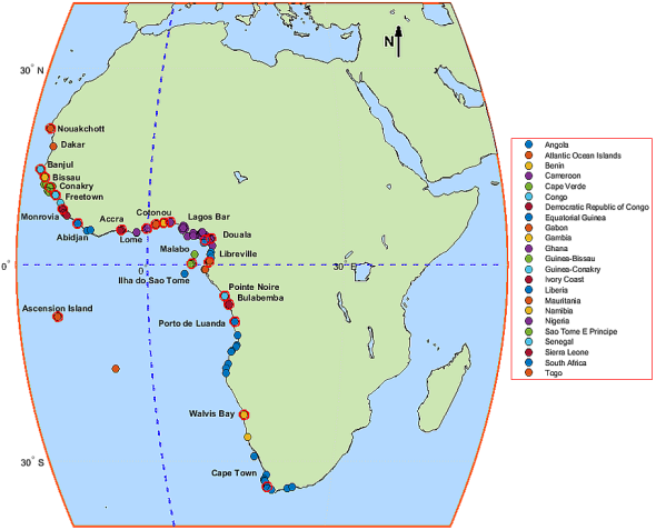
Figure 1. Spatial distribution of the 115 reference ports across 20 West African coastal countries. Full data Table in Table 1.
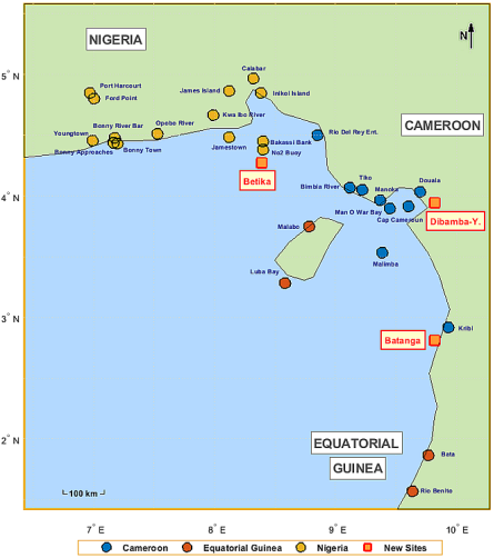
Figure 2. Location of the three test sites Betika, Dibamba-Yassa, and Batanga used for MSL-LAT offset interpolation in the Gulf of Guinea.
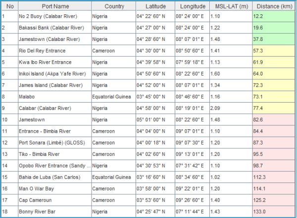
Figure 3. Spatial distribution of the 18 reference stations around Betika (colour-coded by distance: green <30 km, yellow 30-70 km, red >70 km). Source: LSUHydroTide.
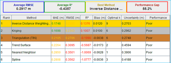
Figure 4. Comparative performance Table of the six interpolation methods for Betika (LOO cross-validation, kmax=12). Source: LSUHydroTide.
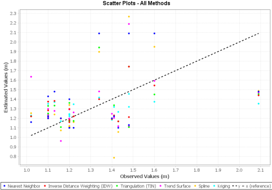
Figure 5. Multi-method scatter plot for Betika (Observed vs. Estimated). Each colour represents a method; the dashed black line=perfect prediction y=x. Source: LSUHydroTide.
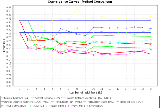
Figure 6. MAE and RMSE convergence curves as a function of the number of neighbours k for the six methods at Betika. Solid lines=MAE, dashed lines=RMSE. Source: LSUHydroTide.
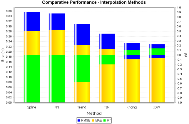
Figure 7. Comparative performance chart of the six interpolation methods at Betika (RMSE in blue, MAE in orange, R² in green on secondary axis). Source: LSUHydroTide.
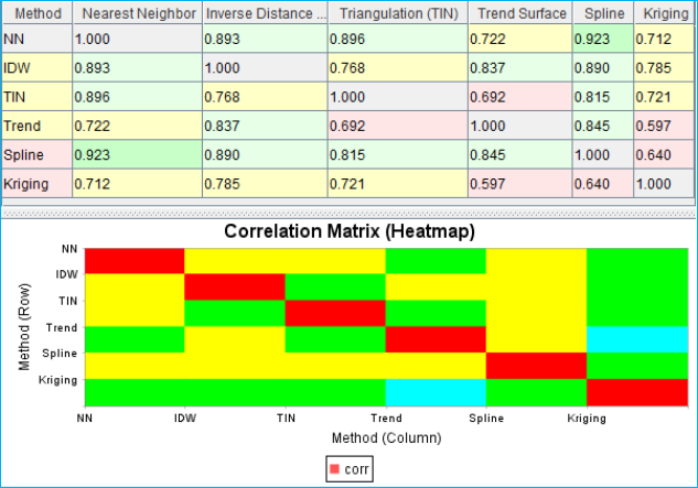
Figure 8. Inter-method correlation matrix heatmap at Betika (red=strong, yellow=weak/negative). Source: LSUHydroTide.
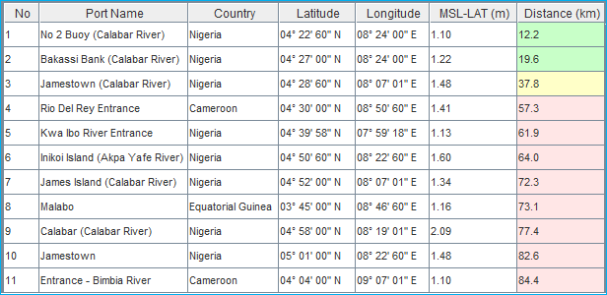
Figure 9. Stations retained for IDW leave-one-out cross-validation at Betika (18-station LOO network, kopt=9). Source: LSUHydroTide.
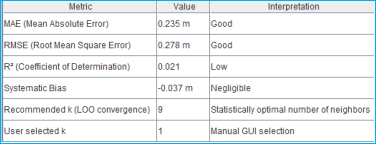
Figure 10. IDW cross-validation evaluation metrics at Betika: MAE=0.1748 m, RMSE=0.2295 m, R²=0.1376, bias=+0.012 m, kopt=9. Source: LSUHydroTide.
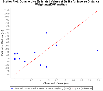
Figure 11. Observed vs. Estimated scatter plot for the IDW method in cross-validation at Betika. The red dashed line represents perfect prediction y=x. Source: LSUHydroTide.
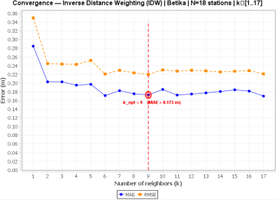
Figure 12. MAE and RMSE convergence curve as a function of k for the IDW method at Betika. The red point marks kopt=9. Source: LSUHydroTide.
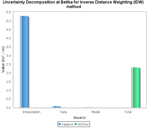
Figure 13. Uncertainty source decomposition for the IDW method in cross-validation at Betika. The dominance of σᵢ² (spatial configuration) is overwhelming. Source: LSUHydroTide.
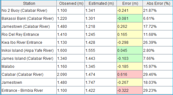
Figure 14. Station-by-station performance for the IDW method at Betika (error <15 cm=green, 15-30 cm=yellow, >30 cm=red). Source: LSUHydroTide.
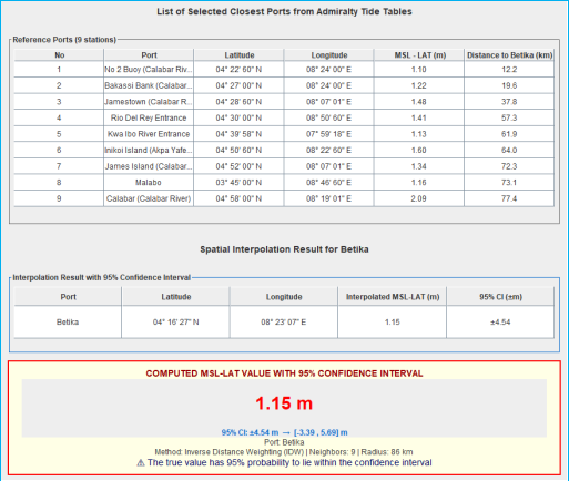
Figure 15. Spatial interpolation result (IDW method, kopt=9) for the Betika site: estimated MSL-LAT offset=1.147 m. Source: LSUHydroTide.
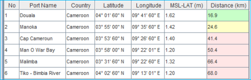
Figure 16. Spatial distribution of the 6 reference stations around Dibamba-Yassa (colour-coded by distance). Source: LSUHydroTide.
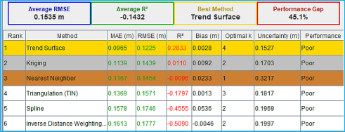
Figure 17. Comparative pesrformance Table of the six interpolation methods for Dibamba-Yassa (leave-one-out cross-validation, kmax=12). Source: LSUHydroTide.
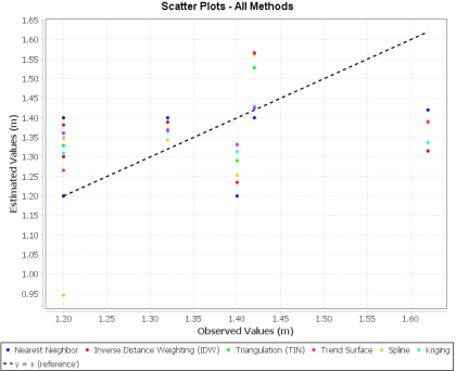
Figure 18. Multi-method scatter plot for Dibamba-Yassa (Observed vs. Estimated). The tendency to underestimate for Douala (1.62 m) is visible for most methods. Source: LSUHydroTide.
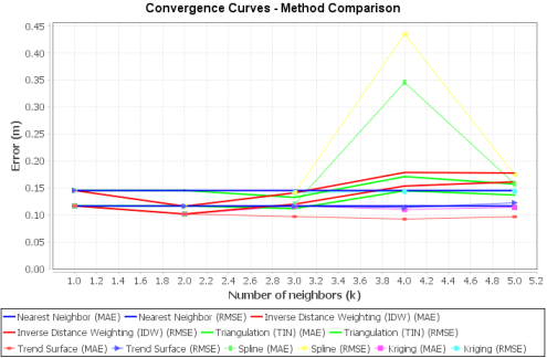
Figure 19. MAE and RMSE convergence curves as a function of k for the six methods at Dibamba-Yassa. Rapid Kriging convergence (kopt=2) and Trend Surface optimum at kopt =4 are noteworthy. Source: LSUHydroTide.
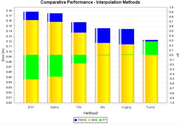
Figure 20. Comparative performance chart at Dibamba-Yassa (RMSE, MAE, R²). The tight hierarchy reflects low spatial variability of the MSL-LAT field in the estuary. Source: LSUHydroTide.
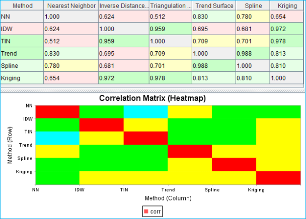
Figure 21. Inter-method correlation matrix heatmap at Dibamba-Yassa. Source: LSUHydroTide.
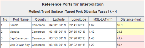
Figure 22. Stations retained for Trend Surface leave-one-out cross-validation at Dibamba-Yassa (4 stations, 56 km radius). Source: LSUHydroTide.
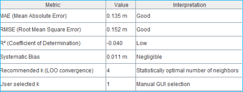
Figure 23. Trend Surface dedicated cross-validation evaluation metrics at Dibamba-Yassa (4-station sub-network, kopt=4): MAE=0.1354 m, RMSE=0.1516 m, R²=-0.040, bias=+0.011 m.
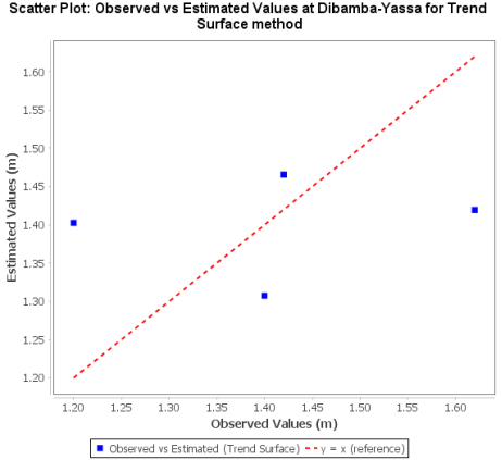
Figure 24. Observed vs. Estimated scatter plot for Trend Surface cross-validation at Dibamba-Yassa. Source: LSUHydroTide.
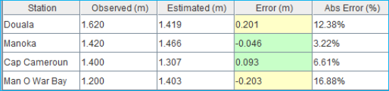
Figure 25. Station-by-station performance for Trend Surface at Dibamba-Yassa. Douala and Man O War Bay concentrate most residual error. Source: LSUHydroTide.
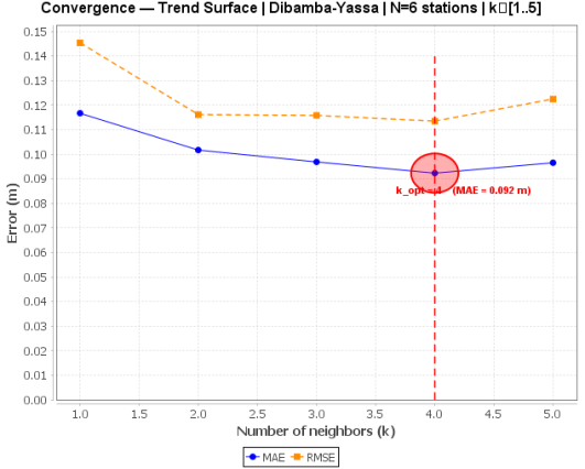
Figure 26. MAE and RMSE convergence curve for Trend Surface at Dibamba-Yassa. Stabilisation from k=4 (kopt, red point). Source: LSUHydroTide.
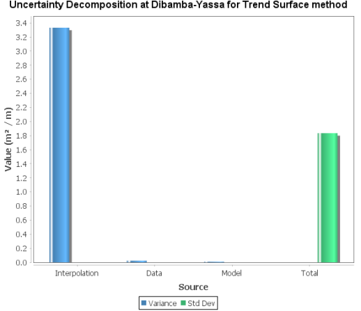
Figure 27. Uncertainty source decomposition for Trend Surface at Dibamba-Yassa. σᵢ² dominance is systematic. Source: LSUHydroTide.
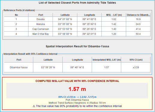
Figure 28. Spatial interpolation result (Trend Surface method, kopt=4) for Dibamba-Yassa: estimated MSL-LAT offset=1.571 m. Source: LSUHydroTide.
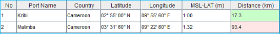
Figure 29. Spatial distribution of the 2 reference stations around Batanga. Total absence of stations in all directions except north-south illustrates the extreme undersampling. Source: LSUHydroTide.
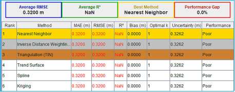
Figure 30. Comparative method Table at Batanga. Perfect identity of metrics for all methods illustrates the mathematical degeneration of the interpolation problem with n=2 stations. Source: LSUHydroTide.
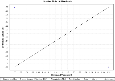
Figure 31. Multi-method scatter plot at Batanga. Perfect superposition of all points and symmetry with respect to y=x illustrate the problem degeneration. Source: LSUHydroTide.
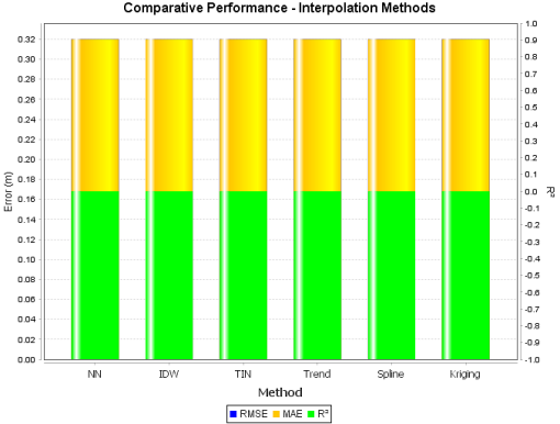
Figure 32. Comparative performance chart at Batanga. Strict identity of RMSE and MAE bars for all methods is the visual signal of degeneration. Source: LSUHydroTide.
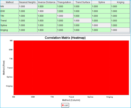
Figure 33. Inter-method correlation matrix heatmap at Batanga. High correlations confirm near-identity of predictions under undersampling. Source: LSUHydroTide.
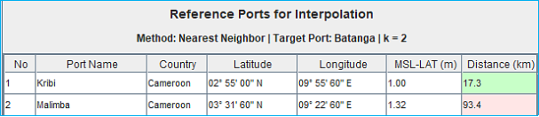
Figure 34. Stations retained for NN cross-validation at Batanga (the 2 only available). Source: LSUHydroTide.
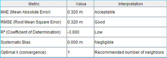
Figure 35. NN evaluation metrics at Batanga: MAE=RMSE=0.320 m, R²=-3.000, bias=0.000 m. Source: LSUHydroTide.
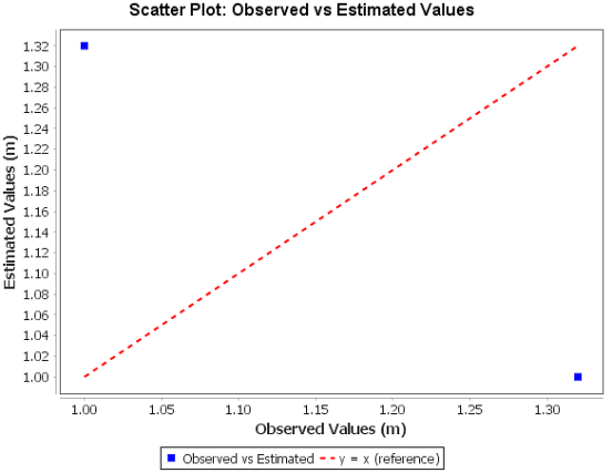
Figure 36. NN scatter plot in cross-validation at Batanga: two symmetric points, no interpolative information. Source: LSUHydroTide.
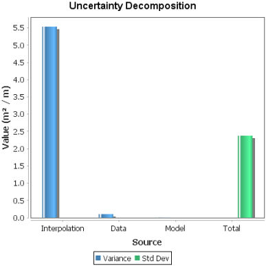
Figure 37. Uncertainty decomposition at Batanga. Near-total dominance of σᵢ² (>98%) shows the problem is entirely governed by network geometry. Source: LSUHydroTide.
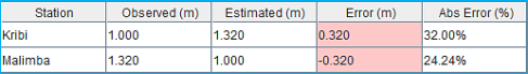
Figure 38. Station-by-station performance for NN at Batanga. The two errors (32% and 24%) reflect only the gap between the two available values. Source: LSUHydroTide.
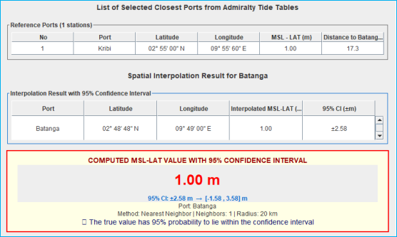
Figure 39. Spatial interpolation result (NN method) for Batanga: MSL-LAT offset=1.00 m (value from Kribi, nearest station at 17.3 km). Source: LSUHydroTide.
Information