Nonintrusive Model Order Reduction Theory in a Fixed Size Domain with Particle in Fluid Flow Application

Seyed Mahdi Razavi; Zeinab Zargar; Syed Farouq-Ali; Mohamed Soliman

doi:doi:10.11648/j.sdenergy.20260101.12

Research Article |

| Peer-Reviewed

Nonintrusive Model Order Reduction Theory in a Fixed Size Domain with Particle in Fluid Flow Application

Seyed Mahdi Razavi, Zeinab Zargar^*

, Syed Farouq-Ali

, Mohamed Soliman

Published in Science Discovery Energy (Volume 1, Issue 1)

Received: 4 December 2025 Accepted: 15 December 2025 Published: 25 February 2026

Views: Downloads:

Download PDF

Share This Article

Twitter
Linked In
Facebook

Abstract

High-fidelity numerical simulation of particle-in-fluid systems is critical for engineering applications such as proppant transport in hydraulic fracturing, cuttings transport in drilling, and fluidization processes, but its practical use is often limited by the high computational cost of Eulerian–Lagrangian (CFD (Computational Fluid Dynamics)–DEM (Discrete Element Method)) methods. Although reduced-physics approaches such as Eulerian–Eulerian models offer faster solutions, they typically sacrifice accuracy by oversimplifying particle dynamics. This work introduces a new nonintrusive Reduced Order Modeling (ROM) strategy that integrates Proper Orthogonal Decomposition (POD) with a previously developed nonintrusive model-order reduction framework to achieve substantial computational acceleration while preserving the fidelity of CFD–DEM simulations. Snapshot-based POD is used to extract dominant flow and particle-motion modes from high-resolution simulations, enabling projection operators that reduce the system dimension by two to three orders of magnitude without modifying the underlying solver. Nonintrusive serial and parallel bridges are constructed to link system states along and across trajectories in input space, allowing nonlinear behavior to be retained while enabling rapid prediction. Additional speed-ups are achieved by projecting these bridges into reduced space, resulting in a ROM–ROM framework. The method is validated using a particle–fluid gas blower model with 3,151 particles and a 12,604-dimensional state space. Snapshot data from four simulations are used to construct reduced bases for particle position and velocity, with 30 POD modes preserving approximately 80–85% of system energy. Predictions for a new operating condition show excellent agreement between the ROM–ROM model, nonintrusive full-space predictions, and the full CFD–DEM solution. Performance analysis demonstrates that the ROM–ROM approach is approximately 3×10⁵ times faster than the full CFD–DEM simulation and about 40 times faster than the nonintrusive full-space method. These results confirm that combining POD with nonintrusive trajectory-based reduction provides an efficient and accurate framework for accelerating multiphase particle-transport simulations, with even greater potential gains for larger systems. This study represents the first POD-enabled nonintrusive ROM applied to particle-in-fluid systems with a fixed particle count, enabling fast surrogate models suitable for real-time simulation, optimization, and uncertainty analysis in complex engineering workflows.

Published in	Science Discovery Energy (Volume 1, Issue 1)
DOI	10.11648/j.sdenergy.20260101.12
Page(s)	14-30
Creative Commons	This is an Open Access article, distributed under the terms of the Creative Commons Attribution 4.0 International License (http://creativecommons.org/licenses/by/4.0/), which permits unrestricted use, distribution and reproduction in any medium or format, provided the original work is properly cited.
Copyright	Copyright © The Author(s), 2026. Published by Science Publishing Group

Keywords

Particle-in-fluid Flow, Nonintrusive Modeling, Reduced Order Modeling (ROM), Proper Orthogonal Decomposition (POD), Computational Efficiency, Proppant Transport

1. Introduction

Engineering problems dealing with complex physics are increasing in number every day and although the computational power and accessibility to high performance computers are increasing, simulation run times for such computationally intensive processes are holding back engineers from investigating the system behaviour as they wish. One way of tackling computation time is to reduce physics and obtain an approximate solution by simplifications and assumptions. This is widely used in many engineering disciplines and is acceptable when reduced physics model can capture the major characteristics of the system behaviour.

The problem we are focusing on in this work is flow of solid particles in fluid which has many applications across different engineering disciplines including petroleum engineering like proppant transport in hydraulic fractures or flow of cuttings in mud during drilling. Daneshy’s work in 1978 is an example of a reduced physic modeling in which Eulerian – Eulerian approach is used for both solid and fluid and they are treated at the same scale

[2]

. These approaches are fast but suffer from improper physics and high dispersion effect due to averaging solid properties to upscale them to the fluid scale. More accurate and recently developed approaches that are Eulerian – Lagrangian schemes that treat solid and fluid in different scales but require an extensive computation power and time

[10]

. The above solutions are widely apart, as one offers a fast but vague solution, and the other offers a very slow but accurate one. A desired solution is one that can predict the system’s behaviour within reasonable accuracy and computation time. The following sections discuss the methodology of implementing such a solution and an example will also be presented to show how it works for a particle-in-fluid flow system.

2. Methodology

2.1. Reduced Order Modeling (ROM)

Reduced order modeling originally known as Model Order Reduction (MOR), is another solution. ROM was first developed in the field of system control to reduce the complexity of a dynamic system while preserving the input–output characteristic behavior as much as possible. Later, it captured the attention of mathematicians and researchers in the field of numerical simulation and today is a flourishing area of research in mathematics, physics, and engineering.

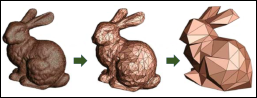
As a solution to computation time and storage capacity for complex processes, ROM captures the essential features of a structure and produces reliable outcomes with sufficient accuracy. In this way, it is even possible to have online predictions for the system behavior within acceptable calculation time to optimize the system. Figure 1, taken from Harvard University – Microsoft research, shows a conceptual schematic of ROM. It shows that sometimes less details may be required to describe a model, just like the rabbit in the Stanford Bunny graphical example that can be recognized with a few facets. Although this example does not reflect the mathematical operations behind the ROM, it is a very simple graphical example to demonstrate the whole idea of reduced order modeling.

Download: Download full-size image

Figure 1. Stanford Bunny Graphical Example to Demonstrate the Overall Idea of REDUCED Order Modeling (ROM).

Approximating a function by a few trigonometrical functions was introduced by Fourier in 1807. Padé in 1890 introduced the Padé approximation which approximates a function by the ratio of two polynomials. These can be considered as the first examples of mathematical model reduction. In linear algebra, Lanczos method was among the first who tried to reduce a matrix in tridiagonal form in 1950

[8]

. Around the same time, in 1951, a paper by Arnoldi was published in which he explained how a smaller matrix can be a good approximation of a larger one

[1]

. But it was not until 80s and 90s of the last century that fundamental methods of ROM were published.

In 1981, Truncated Balanced Realization (TBR) method was introduced by Moore

[9]

which was followed by Glover’s work with Henkel-Norm method in 1984

[6]

. Proper Orthogonal Decomposition (POD) was introduced by Sirovich in 1986

[19]

. Asymptotic Waveform Evaluation (AWE) was published by Pillage in 1990

[12]

as a reduction method using Padé approximation and in 1993, Freund proposed his Padé via Lancsoz (PVL) method

[4]

There are many other old and new ROM methods and reviewing all of them is beyond the scope of this study. In the following subsection, the Krylov subspace methods will be briefly reviewed as they form the foundation of reduced space. Then, the rest of the section will cover the projection base method in depth since this is the method used in this research work.

2.2. Krylov Subspace Methods

Krylov subspace methods are those methods that try to find the “best” approximate solution for a linear set of equation (

A \vec{x} - \vec{b} = 0

) in a Krylov subspace. The basic idea is simple to explain. Since

\vec{b}, \vec{x} \in R^{n}

are vectors in a n-dimensional space, it can be claimed that vectors in the set of

\{{\vec{v}}_{k} = A^{k} \vec{b} | k = 0, 1, 2, \dots\}

are also in the same space. If the first n+1 of these vectors are considered, it is known that they are dependent because in a n-dimensional space, there are only n independent vectors. Therefore, there is a set of coefficients that satisfy

\sum_{k = 0}^{n} α_{k} {\vec{v}}_{k} = \sum_{k = 0}^{n} α_{k} A^{k} \vec{b} = 0 .

(1)

The coefficients,

α_{k}

, can be any real number and at least two of them are non-zero. If

α_{m}

is the first non-zero coefficient, then the above equation can be rewritten as

α_{r} A^{r} \vec{b} = - \sum_{k = m + 1}^{n} α_{k} A^{k} \vec{b} .

(2)

Because

A^{- 1}

exists, both sides can be multiplied by

{(A^{- 1})}^{r - 1}

resulting in

\vec{x} = A \vec{b} = - \sum_{k = r + 1}^{n} \frac{α_{k}}{α_{r}} A^{k - r + 1} \vec{b} .

(3)

The above equation tells us that the solution

\vec{x}

exists in a subspace of the space spanned by

{\vec{v}}_{k}

vectors. In addition, if there are small values of

α_{k}

that can be ignored, the solution can be approximated with a smaller number of

{\vec{v}}_{k}

vectors as

\vec{x} = A \vec{b} \approx - \sum_{k = 0}^{r - 1} β_{k} A^{r} \vec{b} .

(4)

This equation constructs a subspace called Krylov subspace defined as

K_{r} (A, \vec{b}) = \{{\vec{v}}_{k} = A^{k} \vec{b} | k = 0, 1, \dots, r - 1\} .

(5)

Now the question is how to decide for the “best” approximation. Below are the main categories:

1) Minimizing residual

\vec{r} = A \vec{x} - \vec{b}

in Krylov subspace

K_{r} (A, \vec{b})

(CG).

2) Minimizing residual second norm

{‖\vec{r} = A \vec{x} - \vec{b}‖}_{2}

in Krylov subspace

K_{r} (A, \vec{b})

. (Generalized Minimal RESidual (GMRES), MINimal RESidual (MINRES)).

3) Minimizing residual

\vec{r} = A \vec{x} - \vec{b}

in a different Krylov subspace

K_{r} (A^{T}, \vec{b})

(BiCG).

4) Minimizing the error of estimation for

\vec{x}

in Krylov subspace

K_{r} (A, \vec{b})

(SYMmetric Lanczos Q-iteration (SYMMLQ)).

Table 1 summarize all the methods used in Krylov subspace reduction.

Table 1. Summary of Krylov Subspace Methods.

Method

System Specification

Introduced by

Lancsoz / PVL

Hermitian

Lancsoz

[8]

/ Feldman

[4]

Arnoldi / PRIMA

Non-Hermitian

Arnoldi / Odabasioglu

[1]

Conjugate Gradient (CG)

Symmetric positive definite

Hestenes (1952)

[7]

MINRES / SYMMLQ

Symmetric indefinite

Paige (1975)

[11]

GMRES

Non-Symmetric

Saad (1986)

[17]

Bi-Conjugate Gradient (BiCG)

Non-Symmetric

Fletcher (1976)

[5]

2.3. Proper Orthogonal Decomposition (POD)

Proper orthogonal decomposition is a projection-based method meaning that the reduced space is a projection of the Full Order Model (FOM) space using a transfer function. This method is popular in Computational Fluid Dynamic (CFD) applications and is gaining popularity among all other engineering disciplines including system controls as well. The strongest advantage of the POD method is its applicability to nonlinear Partial Differential Equations (PDEs)

[13, 14]

The basic underlying idea of the POD method is that the response of a system at a given time contains all the characteristics and essential behaviour of that system. So, POD collects snapshots of the system at various times and extracts the most important aspects of the behavior in the output, or in the state variables, and preserves those by constructing a reduced space from those snapshots in which output, or state variables, can be estimated with reasonable accuracy.

Finding an orthonormal basis for a reduced order space is an important part of the POD approach. Therefore, in the followings some basics of the POD approach like; projection, determining a n-dimensional space and its orthonormal basis, and eigenvalue problems will be reviewed briefly. Then, POD will be explained in more detail using these basics.

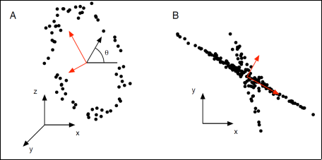
2.3.1. Normal and Oblique Projection

Considering two vectors of

\vec{x} \in R^{n}

and

\vec{y} \in R^{m}

, a matrix of real numbers like

A \in R^{m \times n}

can act as a transformation or linear mapping matrix between the two vectors if

\vec{y} = A \vec{x} \leftrightarrow A : R^{n} \mapsto R^{m} \leftrightarrow y = A (x) .

(6)

With the transformation of

\vec{x}

\vec{y}

as in the above,

\vec{y} = A \vec{x}

, each row of A can be considered as vectors that m-dimensional space of

\vec{y}

is spanning over and each column of A can be considered as vectors that n-dimensional space of

\vec{x}

is spanning over. As the left multiplication of a matrix with a vector is usually used throughout this work, these two interpretations of linear mapping frequently will be used too.

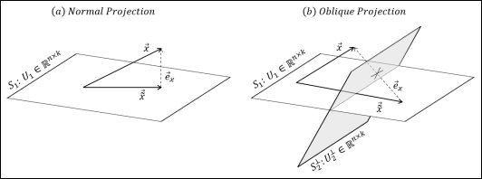
Figure 2 shows a schematic of normal and oblique projections of a vector

\vec{x} \in R^{n}

\vec{\hat{x}} \in R^{k}

. Assuming space

S_{1}

spans over a full-column rank matrix

U_{1} \in R^{n \times k}

and the normal space to

S_{2}

S_{2}^{⊥}

, spans over full-column rank matrix of

U_{2}^{⊥} \in R^{n \times k}

, one can write the equations below for the definition of normal and oblique projections:

\{\begin{matrix} \vec{\tilde{x}} = [U_{1} {(U_{1}^{T} U_{1})}^{- 1} U_{1}^{T}] \vec{x} = Π_{U_{1}, U_{1}} \vec{x}, Normal Projection \\ \vec{\tilde{x}} = [U_{1} {({U_{2}^{⊥}}^{T} U_{1})}^{- 1} {U_{2}^{⊥}}^{T}] \vec{x} = Π_{U_{1}, U_{2}^{⊥}} \vec{x}, Oblique Projection \end{matrix} .

(7)

Download: Download full-size image

Figure 2. Normal and Oblique Projections.

2.3.2. Gram-Schmidt Orthonormalization

A n-dimensional space can be defined with a set of independent vectors like

\{{\vec{v}}_{k} | k = 1, 2, \dots, n\}

, similar to what was defined for a Krylov subspace. As in the example of Krylov space, these vectors are not orthogonal, meaning that there are not two vectors that can satisfy:

{\vec{v}}_{i} . {\vec{v}}_{j} = 0, i \neq j

. Now if the

V = [{\vec{v}}_{j} | j = 1, \dots, n]

matrix is constructed, this matrix is called “orthonormal” if it satisfies:

V . V^{T} = I_{n}

Gram-Schmidt process is a procedure that converts a non-orthonormal basis matrix into an orthonormal one. This conversion has many benefits resulting from the above identity and will be used throughout this work. The procedure is simple and follows

{\vec{u}}_{k} = {\vec{v}}_{k} - \sum_{j = 1}^{k - 1} ({\vec{v}}_{k} . {\vec{u}}_{j}) {\vec{e}}_{j}, {\vec{u}}_{1} = {\vec{v}}_{1}, {\vec{e}}_{i} = \frac{{\vec{u}}_{i}}{|{\vec{u}}_{i}|} .

(8)

Applying the above equation on

V = [{\vec{v}}_{j} | j = 1, \dots, n]

will result in

E = [{\vec{e}}_{j} | j = 1, \dots, n]

which will satisfy:

E . E^{T} = I_{n}

2.3.3. Eigenvalue Methods

Eigenvalue methods are those methods that solve for eigenvalues

\{λ_{i} | i = 1, 2, \dots, n\}

of a matrix

A \in R^{n \times n}

in an eigenvalue problem;

A \vec{v} = λ \vec{v}

in which

\{{\vec{v}}_{i} | i = 1, 2, \dots, n\}

are called eigenvectors corresponding to eigenvalues. The eigenvalue problem of

(A - λI) \vec{v} = 0

can be solved by direct or iterative methods. Arnoldi, QR decomposition and Singular Value Decomposition (SVD) are among those eigenvalue iterative methods that are used extensively in ROM applications. Arnoldi and QR decomposition use Gram-Schmidt type algorithm to create a sequence which will converge into eigenvalues. SVD is not directly an eigenvalue algorithm, but it is used in POD in a way that it results in determining eigenvalues, therefore it will be explained that how SVD works and how it will produce eigenvalues since its basics will be used in this research work.

SVD algorithm factorizes a general rectangular matrix like

A \in R^{n \times m}

into three matrices as

A = U Σ V^{T} : \{\begin{matrix} U \in R^{n \times n} \\ Σ \in R^{n \times m} \\ V \in R^{m \times m} \end{matrix} .

(9)

U \in R^{n \times n}

is an orthonormal matrix that can be a basis for an n-dimensional space.

Σ \in R^{n \times m}

is a diagonal matrix containing singular values of A which are square root of non-negative eigenvalues of A (

σ_{i} = \sqrt{λ_{i}}

). The number of non-zero singular values in this diagonal matrix is equal to the rank of A.

V \in R^{m \times m}

is an orthonormal matrix that can be a basis for an m-dimensional space.

A very useful property of the singular value decomposition of Equation (9) is the result of A^TA or AA^T as shown in equations below:

\{\begin{matrix} A^{T} A = {(U Σ V^{T})}^{T} (U Σ V^{T}) = VΣ U^{T} U Σ V^{T} = {V Σ}^{2} V^{T} \\ A A^{T} = (U Σ V^{T}) {(U Σ V^{T})}^{T} = U Σ V^{T} V^{T} Σ U^{T} = U Σ^{2} U^{T} \end{matrix} .

(10)

Multiplying both sides of the AA^T (or similarly for A^TA) by U gives

(A A^{T}) U = (U Σ^{2} U^{T}) U = U Σ^{2} .

(11)

The above equation indicates that all eigenvalues of

A A^{T}

reside in

Σ^{2}

. This property will be used later for the POD method and the application. At this point all the prerequisites to explain the POD method have been covered properly. In the following sections, Proper Orthogonal Decomposition (POD) in particle-in-fluid flow, which has never been done before, will be covered and it will be shown how to combine this technique with the previous nonintrusive formulation introduced Razavi in 2022 to build a predictive model that runs several orders of magnitude faster than the full order model

[15]

. Therefore, the POD steps introduced before will be reviewed again but more in the context of particle-in-fluid flow. The POD in this study will be performed in three major steps and then will be combined with the nonintrusive method explained by the author to establish a new ROM method that can reduce the computation time significantly. The resulting formulation is then applied to a solid blower example to prove the concept.

2.4. Data Construction in Full Space

The reduced space (reduced order space) is hidden inside snapshot data taken in the full space. A snapshot can be defined as a vector of primary variables or state variables taken at a certain time while simulating or measuring a process. The snapshots data has seen the system behavior and experienced the state variables variations. When state variables show erratic variations and change significantly during a run, a wider distribution of numbers and higher standard deviations is observed. Such a system needs more principal components to be explained in comparison to a system that does not show much of variation in its state variables.

The above general rule applies to each individual state variable since some variables may experience wider changes than others. This becomes clearer with an example. In a container, particles positions (state variables x and y in a two-dimensional model) cannot go beyond the container limits, but the velocity components can go from a very small value or zero to a very high value and can experience a wide variation. This is the common problem of scaling and normalization is used in this study as the solution and all calculations are performed on normalized variables. Therefore, rather than the scale of changes, the concern is more about the rate of changes. Particle location from one time step to another does not change widely because time step does not allow a particle to travel far but velocity, which is mostly dictated by collisions, can change erratically. This behavioral difference in state variables forces us to separate variables and find a reduced space for each separately instead of finding one reduced space for all state variables. This is a common practice in most POD applications.

Finding one reduced space for each state variable results in some changes in the shape of the equations and matrices that were introduced before. The transformation equation between full and reduced order spaces is

\vec{x} = Φ \vec{\hat{x}}, \vec{x} \in R^{N}, Φ \in R^{N \times R}, \vec{\hat{x}} \in R^{R}, N ≫ R, N = N_{p} \times N_{s} .

(12)

Here

\vec{x}

and

\vec{\hat{x}}

are state variable is full and reduced spaces respectively.

N

is the number of state variables in any snapshot in full space dimension.

N_{p}

is the number of particles in any snapshot,

N_{s}

is the number of state variables for each particle and

R

is the number of principal components in any snapshot.

The above equation is written for a case that all state variables are reduced using the same transformation matrix or basically to the same reduced space. In this case, the ordering of state variables inside

\vec{x}

becomes irrelevant and

Φ

will be shaped in a way that preserves the ordering between reduced space and full space. But how will these equations change or how each snapshot state variable vector is formed if there is a different transformation matrix for each state variable? Equation (13) shows how the transformation equation will look like when there is one transformation matrix for each state variable.

\vec{x} = [\begin{matrix} Φ^{x} \\ Φ^{y} \\ Φ^{u_{x}} \\ Φ^{u_{y}} \end{matrix}] \vec{\hat{x}}, \vec{x} = |\begin{matrix} x_{1} \\ ⋮ \\ x_{N_{p}} \\ y_{1} \\ ⋮ \\ y_{N_{p}} \\ u_{x 1} \\ ⋮ \\ u_{x N_{p}} \\ u_{y 1} \\ ⋮ \\ u_{y N_{p}} \end{matrix}

(13)

Where

Φ^{x}

Φ^{y}

Φ^{u_{x}}

and

Φ^{u_{y}}

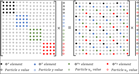
are projection matrices for position and velocity x and y components respectively.

As shown in the above equation, the snapshot state vector is constructed starting with all x values first, then all y values and so on. There is another way of configuration

\vec{x}

\vec{x} = |\begin{matrix} x_{1} \\ y_{1} \\ u_{x 1} \\ u_{y 1} \\ x_{2} \\ y_{2} \\ ⋮ \\ ⋮ \\ x_{N_{p}} \\ y_{N_{p}} \\ u_{x N_{p}} \\ u_{y N_{p}} \end{matrix} .

(14)

The projection/transformation matrix format in Equation (13) is easier to build, but the state vector configuration in Equation (14) is more convenient to work with. Computationally, the projection matrix is built once, but state variable vectors are used many times. So, it is preferred to continue with a convention that is easier to implement in terms of configuring state variable vectors. This requires reconfiguration of the projection matrix from its convenient form in Equation (13). Figure 3 shows a schematic of this reconfiguration for a small example.

Download: Download full-size image

Figure 3. Reconfiguration of the Projection Matrix in Order to be Consistent with State Variable Vector Ordering.

Another major concern in constructing the projection matrix from snapshot data is the number of available data points. It is known that finding the reduced space is an eigenvalue problem represented by

[15].

R {\vec{ψ}}_{i} = λ_{i} {\vec{ψ}}_{i}, R = \frac{1}{N_{snt}} X X^{T}, {\vec{ψ}}_{i} \in R^{N}, X \in R^{N_{sn} \times N} .

(15)

Where

X

is the matrix of snapshot data,

{\vec{ψ}}_{i}

is eigenvectors,

λ_{i}

is eigenvalues,

N_{snt}

is total number of snapshots used in building X and

N

is the number of state variables in any snapshot – Full space dimension.

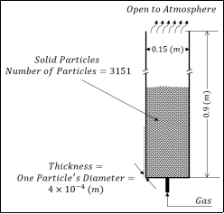
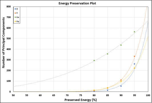
Based on the above equation, matrix R has the size of N_sn×N_sn. Such a matrix has N_sn number of eigenvalues and eigenvectors, meaning that maximum number of principal components explaining the variation in state variables can reach N_sn. This shows the importance of the available number of snapshots in building snapshot matrix X. In the gas blower example which will be presented later as a case study, there are 3151 particles and four state variables for each particle which makes the size of state variable vector for a snapshot 12,604. Therefore, in each snapshot there is a 12604-dimensional vector in full space. If 10 snapshots are gathered, there will be an ‘R’ matrix with size of 10×10 and a reduced space that at its maximum has 10 dimensions. In other words, a 12,604-dimensional space is being explained with only 10 principal components! It is possible to do it mathematically even with less than 10 number of components, but when the number of principal components is low, each of the corresponding eigenvalues carries a big weight in preserving the system energy. This means that if one is dropped, suddenly 10% or 25% of the system energy will be lost. Therefore, it is preferable to increase the number of available components to at least 20 or 30 so that each does not carry a big weight in preserving the system energy and the smallest ones may preserve less than 1% of the energy and can be easily ignored.

The above concept enforces using at least 20 to 30 snapshots to build the snapshot data matrix X. Two families of snapshots are available. First, those that are along the closest run (available simulations or measurements) trajectory which is the run that its location in the input space is the closet to the prediction run (simulation) and second, those that are available in the neighboring runs which are usually runs that are not as close but can be used to calculate the required spatial gradients

[15]

. Therefore, the total number of available snapshots will be

N_{snt} = N_{sn} \times (N_{r} + 1) .

(16)

Where

N_{sn}

is the number of available snapshots in the closest run and

N_{r}

is the number of neighboring runs.

Usually more than 10 snapshots are selected among the available frames and there are commonly at least 3 neighboring runs, so maximum number of components can easily reach 40. But it is always essential to keep track of the available data and how principal components are limited to it. Equation (16) determines the maximum number of principal components, and one can judge and act accordingly to provide enough snapshots if that number is low.

Snapshot data matrix, X, includes all state variable vectors for all N_snt number of snapshots and can be expanded as

X = [\begin{matrix} x_{1}^{1}, y_{1}^{1}, u_{x 1}^{1}, u_{y 1}^{1}, x_{2}^{1}, y_{2}^{1}, u_{x 2}^{1}, \dots, \dots, x_{N_{p}}^{1}, y_{N_{p}}^{1}, u_{x N_{p}}^{1}, u_{y N_{p}}^{1} \\ x_{1}^{2}, y_{1}^{2}, u_{x 1}^{2}, u_{y 1}^{2}, x_{2}^{2}, y_{2}^{2}, u_{x 2}^{2}, \dots, \dots, x_{N_{p}}^{2}, y_{N_{p}}^{2}, u_{x N_{p}}^{2}, u_{y N_{p}}^{2} \\ ⋮ \\ x_{1}^{N_{snt}}, y_{1}^{N_{snt}}, u_{x 1}^{N_{sn t}}, u_{y 1}^{N_{snt}}, \dots, \dots, x_{N_{p}}^{N_{snt}}, y_{N_{p}}^{N_{snt}}, u_{x N_{p}}^{N_{snt}}, u_{y N_{p}}^{N_{snt}} \end{matrix}] \in R^{N_{snt} \times N} .

(17)

When the above matrix is built from all the available snapshots, the projection or transformation matrix is extracted from it which is the topic of the next section.

2.5. Singular Value Decomposition (SVD)

The transpose of the snapshot data matrix,

X^{T}

, can be considered as a collection of vectors (N_snt of them) in a full order N-dimensional space (N=N_p×N_s). Any arbitrary unit vector in the reduced order N_snt-dimensional space can be specified as

{█ (X^T . ψ ⃗_i = c_i 1 φ ⃗_1 + c_i 2 φ ⃗_2 + \dots + c_ij φ ⃗_j + \dots + c_iN φ ⃗_N = [φ ⃗_1, \dots, φ ⃗_N] . | █ (c_i 1 @ ⋮ @ c_iN) = Φ c ⃗_i ┤ @ @ ψ ⃗_i \in R^(N_snt), X^T \in R^(N \times N_snt), 〖 X^T . ψ ⃗_i \in R^N, φ ⃗ 〗_j \in R^N, c ⃗_i \in R^N) ┤

(18)

The left-hand side of the above equation is a vector in full space and can be written as a linear combination of unit vectors in this N-dimensional space. The above equation can be extended for all unit vectors in the reduced space resulting in

X^{T} . Ψ = ΦC, Ψ \in R^{N_{snt} \times N_{snt}}, Φ \in R^{N \times N}, C \in R^{N \times N_{snt}} .

(19)

In the above equation, C is a coefficient matrix. Because both Ф and Ψ are unitary matrices and orthonormal in their own spaces, both sides cab be multiplied from right by Ψ^T to obtain

X^{T} . I_{N_{snt}} {= X}^{T} = ΦC Ψ^{T} .

(20)

The above equation is the well-known form of the singular value decomposition formulation in which any matrix can be decomposed into two orthonormal matrices and one diagonal matrix. Therefore, the coefficient matrix is the same as the diagonal matrix in the singular value decomposition method shown with Σ in equation below.

X^{T} = ΦΣ Ψ^{T}, Σ \in R^{N \times N_{snt}}

(21)

There are many algorithms available for implementing SVD. Based on the matrix type, they are categorized into full SVD and truncated SVD acting on dense and sparse matrices, respectively. In this work, snapshot data matrices are dense matrices because there are many data points available for state variables and they are mainly non-zero. In terms of algorithms, SVD methods are categorized into QR decomposition based and Divide and Conquer based algorithms. Finally, in terms of available resources, libraries, and implementations, there are many libraries that are widely used by researchers and developers like Linear Algebra PACKage (LAPACK), Scalable Linear Algebra PACKage (ScaLAPACK), Parallel Linear Algebra Software for Multicore Architectures (PLASMA), Distributed Parallel Linear Algebra Software for Multicore Architectures (DPLASMA), Matrix Algebra on GPU and Multicore Architectures (MAGMA) and Software for Linear Algebra Targeting Exascale (SLATE) providing basic functionalities as well as addressing issues like bounded memory, parallelization and using GPU accelerators. In 2018, Dongara documented a comprehensive review of all SVD theories and algorithms and compared the performances of the above-mentioned libraries

[3]

. Going deeper through the singular value decomposition and its theory or implementation is out of the scope of this work, but it is proper to mention that the standard LAPACK implementation of the SVD is used in this work.

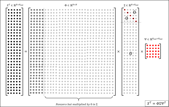
X^T in Equation (21) can be considered as the snapshot data matrix written in its collective vector form. These vectors are now explained by three matrices in the right-hand side of this equation. Figure 4, displays how these matrices are structured. Clearly, none of the unit vectors after N_snt^th column in Ф plays any role in explaining X^T because they are all multiplied by zeros in Σ and are omitted. In addition, all first N_snt vectors in Ф have a corresponding coefficient on the main diagonal of Σ showing their weights in describing X^T. With this understanding it is time to define the reduced space.

Download: Download full-size image

Figure 4. A Schematic of Singular Value Decomposition and the Structure of Resulted Matrices.

2.6. Reduced Space Sizing

The process of finding a reduced space is an optimization process in which it is tried to reduce the error between a vector (state variable vector) and its projection to a minimum. Equation (15) is the problem to solve to find the reduced space. Substituting X in Equation (15) by X^T, which is the transpose of snapshot data matrix, gives

\{\begin{matrix} R {\vec{φ}}_{i} = λ_{i} {\vec{φ}}_{i}, {\vec{φ}}_{i} \in R^{N} \\ R = \frac{X^{T} X}{N_{snt}} = \frac{(ΦΣ Ψ^{T}) {(ΦΣ Ψ^{T})}^{T}}{N_{snt}} = \frac{Φ Σ^{2} Φ^{T}}{N_{snt}} \end{matrix} \to R Φ = \frac{1}{N_{snt}} Φ Σ^{2} .

(22)

The above equation indicates that Ф, which was already found using SVD, is the basis for the reduced space. It is worth mentioning that out of all N available unit vectors in this matrix, there are only N_sntof them that are associated with nonzero eigenvalues. This is the fact that reduces the space dimension from N to the maximum of N_snt. This is consistent with the observation in Figure 4. The importance of each first N_snt directions in Ф depends on its corresponding eigenvalue in Σ. Therefore, the unit vectors are usually sorted based on their corresponding eigenvalues and are added in that order to the reduced space until a certain level of energy preservation is reach based on

E_{POD} = 1 - \frac{Er (r)}{Er (0)} = (\sum_{i = 1}^{r} λ_{i}) / (\sum_{i = 1}^{n} λ_{i}) .

(23)

It was previously mentioned that one transformation matrix (Ф) is prepared for each state variable (x, y, u_x, u_y). Therefore, all the steps described in the above to find and size the reduced space should be repeated for each state variable starting with preparing X_x, X_y, X_ux, X_uy and going through all steps to find Ф_x, Ф_y, Ф_ux, Ф_uy.

2.7. Projection into Reduced Space

When all the transformation matrices are built using SVD, projecting the full space equations into the reduced space can be started. At this point governing equations are required to be multiplied by the transfer functions in order to project the equations in the reduced order space which has a smaller size and solve them there for reduced size state variable. Now, instead of full physics governing equations, nonintrusive equations developed by the author for any physics including particle-in-fluid flow is used to show how the combination can be used for a system with fixed number of particles, like the gas blower example, to decrease the computation time while maintaining an acceptable accuracy.

Based on Razavi’s nonintrusive theory, Equation (24) can reproduce and predict the system behavior based on given runs or measurements for given inputs. In this equation

A_{n}

and

B_{n}

are called serial and parallel bridges and are simply gradients along and perpendicular to the closet available run trajectory in the full space.

\vec{u}

is the input space vector and

Δ \vec{u}

represents the difference in input vectors between the closest run and a neighboring run. The rest of the equation is self-explanatory since it follows the simplest form of the Trajectory Piecewise Linearization (TPWL) proposed by Rewienski in 2003

[16]

{\vec{x}}^{m *}

is the projection of any point like

{\vec{x}}^{m}

along the closet run trajectory and since most of the time the prediction run is close enough to the closest run, they are considered the same, but we keep the general form as

{\vec{x}}^{m + 1} = {\vec{x}}^{n + 1} + A_{n} ({\vec{x}}^{m *} - {\vec{x}}^{n}) + B_{n + 1} Δ \vec{u}, Δ \vec{u} = ({\vec{u}}^{p} - {\vec{u}}^{s}) .

(24)

The projection matrix that was defined and sized in the previous subsection can transfer any state variable vector in the full space to its projection vector in the reduced space by

\vec{x} (t) = Φ \vec{\hat{x}} (t), Φ \in R^{N \times R}, \vec{\hat{x}} \in R^{R}, R \leq N_{snt} .

(25)

Where

\vec{\hat{x}}

is the reduced state variable vector and

R

is reduced space dimension. Substituting the above equation into Equation (24) gives

{Φ \vec{\hat{x}}}^{m + 1} = Φ {\vec{\hat{x}}}^{n + 1} + A_{n} Φ ({\vec{\hat{x}}}^{m *} - {\vec{\hat{x}}}^{n}) + B_{n + 1} Δ \vec{u}, {\vec{x}}^{m *} = {\vec{x}}^{m} - B_{n} Δ \vec{u} .

(26)

Multiplying both sides from the left side by Ф^T gives

{\vec{\hat{x}}}^{m + 1} = {\vec{\hat{x}}}^{n + 1} + ({Φ^{T} A}_{n} Φ) ({\vec{\hat{x}}}^{m *} - {\vec{\hat{x}}}^{n}) + (Φ^{T} B_{n + 1}) Δ \vec{u}, Δ \vec{u} = ({\vec{u}}^{p} - {\vec{u}}^{s}) .

(27)

Defining the reduced serial and parallel bridges finalizes equations in the reduced space as:

\{\begin{matrix} {\vec{\hat{x}}}^{m + 1} = {\vec{\hat{x}}}^{n + 1} + {\hat{A}}_{n} ({\vec{\hat{x}}}^{m *} - {\vec{\hat{x}}}^{n}) + {\hat{B}}_{n + 1} Δ \vec{u}, Δ \vec{u} = ({\vec{u}}^{p} - {\vec{u}}^{s}) \\ {\hat{A}}_{n} = {Φ^{T} A}_{n} Φ, {\hat{A}}_{n} \in R^{R \times R} \\ {\hat{B}}_{n + 1} = Φ^{T} B_{n + 1}, {\hat{B}}_{n + 1} \in R^{R \times I} \end{matrix} .

(28)

Where

{\hat{A}}_{n}

and

{\hat{B}}_{n}

are reduced serial and parallel bridge matrices, respectively. Considering the size of parallel and serial bridges and all vectors in the above equation, the speed gain in calculations can be concluded by comparing it to Equation (24). In the following section the implementation and speed gain will be discussed in further detail to see how much speed is expected to be gained from this nonintrusive model order reduction in terms of computation time.

2.8. Simulation Types

All state vectors and bridges in Equation (28) exist in the reduced space except for the input vector. This vector is very small and there is no need to project it to the reduced space. Working with Equation (28) in its current form requires projecting all vectors into reduced space and storing them for any calculation during the simulation process. This memory consumption is avoided by projecting vectors on the fly and transferring them when they are needed for a calculation. Serial and parallel bridges, on the other hand, are projected and stored in memory because transferring them on the fly many times is computationally expensive especially for the serial bridge that has a considerable size. Applying this implementation technique to Equation (28) will change its form to

{\vec{x}}^{m + 1} = {\vec{x}}^{n + 1} + (Φ {\hat{A}}_{n} Φ^{T}) ({\vec{x}}^{m *} - {\vec{x}}^{n}) + (Φ {\hat{B}}_{n + 1}) Δ \vec{u}, Δ \vec{u} = ({\vec{u}}^{p} - {\vec{u}}^{s}) .

(29)

Clearly in the above equation, it is tried to avoid using full order serial bridge and the reduced one is used instead. This may not be the case for the parallel bridge since it is not as huge as the serial bridge is. For that reason, another version of the above equation is presented as

{\vec{x}}^{m + 1} = {\vec{x}}^{n + 1} + (Φ {\hat{A}}_{n} Φ^{T}) ({\vec{x}}^{m *} - {\vec{x}}^{n}) + B_{n + 1} Δ \vec{u}, Δ \vec{u} = ({\vec{u}}^{p} - {\vec{u}}^{s}) .

(30)

Based on the presented equations (Equation (28), Equation (29) and Equation (30)) for the simulation runs, the simulation process is categorized into three types:

NIM – NIM: This is when the process is simulated based on Equation (28) in which both serial and parallel bridges are calculated using the nonintrusive approach. This simulation happens completely in the full order space and none of the vectors or matrices are projected or stored in the reduced space.

ROM – NIM: This type of simulation is based on Equation (29) in which serial bridges are transferred and stored in the reduced space, but parallel bridges remain in the full order space. None of the state vectors are projected for the reason discussed before.

ROM – ROM: When Equation (30) is used for the simulation in which both serial and parallel bridges are transferred into the reduced space, it is the ROM – ROM case. Again, it is only bridges that are stored in their reduced formats and none of the state variable vectors are stored in the reduced space.

2.9. Speed Gain Discussion

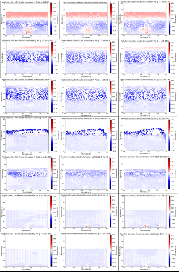
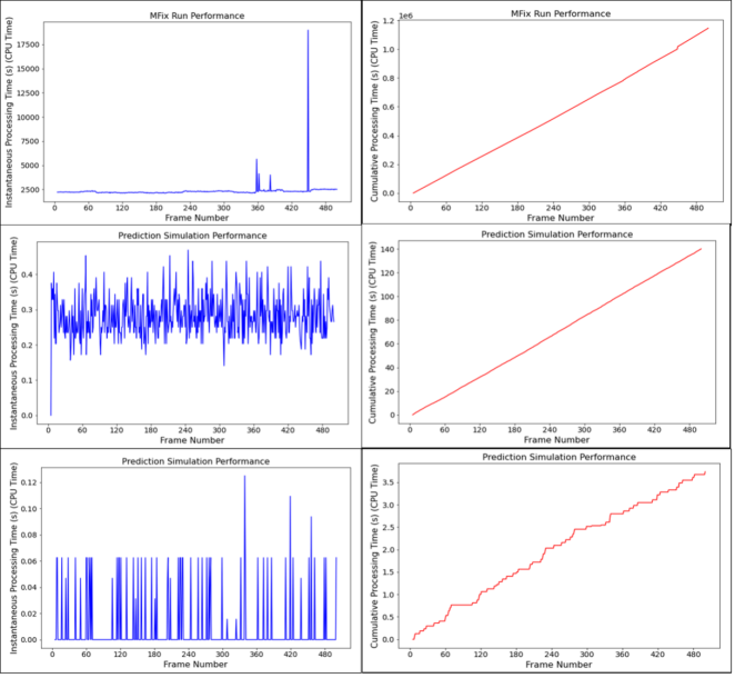
Simulation types were discussed in the above and now the speed gain from each type is reviewed and calculated. It was already shown by the author that using the nonintrusive approach instead of solving full order model and governing equations helps in gaining computation time. Here, the extra speed gain is calculated when model order reduction is added to the nonintrusive approach. Therefore, benchmarking will be against the NIM – NIM simulation process not against the full order solver. The practical speed gain from actual CPU times will be discussed and presented in the results section. What is discussed here is the expected theoretical speed gain relative to the NIM – NIM simulation when the model order reduction is added to it.

All presented simulation formulations are linear algebraic equations with matrix and vector multiplications. A simple approach was taken to calculate the number of operations required for a matrix – matrix or matrix – vector multiplication and it is extended to calculate the number of operations required for a single time step in a simulation process. Then, the results will be compared to see how much speed gain is expected from each simulation type against the NIM – NIM type. To start, it is assumed to have a general matrix (M), and a vector (b). The required order of operations for a matrix – vector multiplication is

\{\begin{matrix} M \in R^{N_{i} \times N_{j}} \\ \vec{b} \in R^{N_{j}} \end{matrix} \to Ο (M \vec{b}) = N_{i} \times (2 N_{j} - 1) ≅ 2 N_{i} N_{j}

(31)

Using Equation (31), terms and operations in simulation type equations are broken into pieces and the required order of operations is calculated for each simulation type equation. Table 2 to Table 4 summarize the calculation steps and order of operations.

Table 2. Required Order of Operations for NIM – NIM Simulation Type.

NIM-NIM Simulation Type
${\vec{x}}^{m + 1} = {\vec{x}}^{n + 1} + A_{n} ({\vec{x}}^{m *} - {\vec{x}}^{n}) + B_{n + 1} Δ \vec{u}, Δ \vec{u} = ({\vec{u}}^{p} - {\vec{u}}^{s})$
Step	Operation	Size	Order
1.	$({\vec{x}}^{m *} - {\vec{x}}^{n})$	$(N \times 1) - (N \times 1)$	$N$
2.	${A_{n} \times Ans}_{1}$	$(N \times N) \times (N \times 1)$	${2 N}^{2}$
3.	$({\vec{u}}^{p} - {\vec{u}}^{s})$	$(I \times 1) - (I \times 1)$	$I$
4.	$B_{n + 1} {\times Ans}_{3}$	$(N \times I) \times (I \times 1)$	$2 NI$
5.	${\vec{x}}^{n + 1} + {Ans}_{2} + {Ans}_{3}$	$(N \times 1) + (N \times 1) + (N \times 1)$	$2 N$
Total=			${2 N}^{2}$

Table 3. Required order of operations for ROM – NIM simulation type.

ROM-NIM Simulation Type
${\vec{x}}^{m + 1} = {\vec{x}}^{n + 1} + (Φ {\hat{A}}_{n} Φ^{T}) ({\vec{x}}^{m *} - {\vec{x}}^{n}) + B_{n + 1} Δ \vec{u}, Δ \vec{u} = ({\vec{u}}^{p} - {\vec{u}}^{s})$
Step	Operation	Size	Order
1.	$({\vec{x}}^{m *} - {\vec{x}}^{n})$	$(N \times 1) - (N \times 1)$	$N$
2.	$Φ^{T} \times {Ans}_{1}$	$(R \times N) \times (N \times 1)$	$2 NR$
3.	${{\hat{A}}_{n} \times Ans}_{2}$	$(R \times R) \times (R \times 1)$	${2 R}^{2}$
4.	${Φ \times Ans}_{3}$	$(N \times R) \times (R \times 1)$	$2 NR$
5.	$({\vec{u}}^{p} - {\vec{u}}^{s})$	$(I \times 1) - (I \times 1)$	$I$
6.	$B_{n + 1} {\times Ans}_{5}$	$(N \times I) \times (I \times 1)$	$2 NI$
7.	${\vec{x}}^{n + 1} + {Ans}_{4} + {Ans}_{6}$	$(N \times 1) + (N \times 1) + (N \times 1)$	$2 N$
Total=			$4 NR$

Table 4. Required order of operations for ROM-ROM simulation type.

ROM-ROM Simulation Type
${\vec{x}}^{m + 1} = {\vec{x}}^{n + 1} + (Φ {\hat{A}}_{n} Φ^{T}) ({\vec{x}}^{m *} - {\vec{x}}^{n}) + (Φ {\hat{B}}_{n + 1}) Δ \vec{u}, Δ \vec{u} = ({\vec{u}}^{p} - {\vec{u}}^{s})$
Step	Operation	Size	Order
1.	$({\vec{x}}^{m *} - {\vec{x}}^{n})$	$(N \times 1) - (N \times 1)$	$N$
2.	$Φ^{T} \times {Ans}_{1}$	$(R \times N) \times (N \times 1)$	$2 NR$
3.	${{\hat{A}}_{n} \times Ans}_{2}$	$(R \times R) \times (R \times 1)$	${2 R}^{2}$
4.	${Φ \times Ans}_{3}$	$(N \times R) \times (R \times 1)$	$2 NR$
5.	$({\vec{u}}^{p} - {\vec{u}}^{s})$	$(I \times 1) - (I \times 1)$	$I$
6.	${\hat{B}}_{n + 1} {\times Ans}_{5}$	$(R \times I) \times (I \times 1)$	$RI$
7.	${Φ \times Ans}_{6}$	$(N \times R) \times (R \times 1)$	$2 NR$
8.	${\vec{x}}^{n + 1} + {Ans}_{4} + {Ans}_{7}$	$(N \times 1) + (N \times 1) + (N \times 1)$	$N$
Total=			$6 NR$

Comparing the operation orders against the NIM-NIM simulation gives

\{\begin{matrix} \begin{matrix} \frac{Ο (NIM - NIM)}{Ο (ROM - NIM)} = \frac{2 N^{2}}{4 NR} = \frac{N}{2 R} \end{matrix} \\ \frac{Ο (ROM - ROM)}{Ο (ROM - NIM)} = \frac{6 NR}{4 NR} = \frac{3}{2} \end{matrix} .

(32)

Usually the full space dimension, N, is 2 to 3 orders of magnitude bigger than the reduced space dimension, R. So, it is expected to see a significant acceleration in calculations from NIM – NIM type to ROM – NIM/ROM – ROM type. The above equation shows that NIM – ROM is faster than ROM – ROM but not significantly, therefore, ROM – ROM simulation type will be used in future benchmarking.

3. Case Study

In this section, the same model used in previous work by the author will be used but the reduced order modeling will be added to the progressive nonintrusive model and results will be presented and discussed. Figure 5 shows a schematic of the solid fluidization bed, which will be also referred to “gas blower” in this study. Design and simulation parameters are listed in Table 5. In this process gas blows to these particles for 5 seconds and the input space consists of gas velocity, gas viscosity and particle density variables forming a 3-dimensional input space. The first goal here is to make sure that the theory developed results in acceptable accuracy comparing to NIM – NIM by reproducing the same prediction run as in the previous work for gas velocity of 41.5 (m/s), gas viscosity of 1.7×10^-5 (Pa.s) and particle density of 2600 (kg/m³). If the accuracy is acceptable, then the computation speeds will be compared to measure the actual speed gain.

Download: Download full-size image

Figure 5. A Schematic of the Gas Blower Model Used in This Study.

Table 5. Parameters Used to Run the Gas Blower Simulations.

Property	Value (unit)
Height	0.9 (m)
Length	0.15 (m)
Depth	0.0004 (m)
Particle density	2700 (kg/m³)
Particle diameter	0.0004 (m)
Gas viscosity	1.8×10^-5 (Pa.s)
Gas velocity	42 (m/s)
Outlet pressure	1 (bar)
Temperature	293.15 (°K)

Results are presented in the same order and manner as appeared in the previous work by the author and the same ranges or target snapshots will be selected to make the comparisons easier. It is worth mentioning that domain decomposition and snapshot reproduction from clustering still happen in the full order space and are not affected by the model order reduction, therefore, those results will not be covered here.

3.1. Reduced Space Construction

Download: Download full-size image

Figure 6. Energy Preservation Plot Showing the Required Number of Principal Components to Preserve a Certain Amount of Energy in the System While Projecting to the Reduced Space.

Download: Download full-size image

Figure 7. A Schematic of Trendless Data in Higher Dimension and Its Equally Strong Principal Components in Lower Dimensional Space

[18]

As mentioned before, the number of particles in the gas blower example is 3151 and each particle has four state variables of x, y, u_x, u_y. So, each snapshot state vector has the dimension of 3151×4=12,604. During each 5 second simulation run in the input space, 495 snapshots were taken to be used. There are three input variables of gas viscosity, gas injection velocity and solid density. This makes the input space 3 dimensional and to define a 3-dimensional input space, it is required to have at least 4 runs including the closest run. Using Equation (16) determines the maximum number of available principal components as 495 × (3+1) =1980, meaning that the full 12,604-dimensional space is explained by a 1980-dimensional reduced space. This number is still very high, and the reduced space dimensions can be reduced furthermore. Figure 6 shows the energy preservation plot prepared for the gas blower example. The required number of principal components drops drastically when the requested energy preservation is decreased from 95% to 90% and so on except for the x-direction velocity component which has a modest decrease. When behaviour like u_x’s trend is observed in Principal Component Analysis (PCA), it indicates that the data does not have strong correlation to be captured by PCA analysis

[18]

. Figure 7 shows a nice schematic of how trendless data may look like in a 3-dimensional space that any of its 2-dimensional representations is equally strong. This means that each component carries the same weight in the system energy.

With this better understanding of the u_x trend and the reason behind it, one can decide on the size of the reduced space. All other state variables show almost 85% energy preservation using 30 components, so 30 is used for the number of components for all state variables and building the projection matrix.

3.2. Prediction Run

There are usually two approaches to evaluate the response accuracy of a proxy model. One is to ask the model to reproduce the closest run in the input space and the other is to ask the model to predict a run which it was blind to and do a blind test. Generally, the proxy model accuracy is higher in a reproduction run compared to prediction run. In other words, if the prediction run accuracy is acceptable, it is valid to assume that reproduction run has an acceptable accuracy too. Therefore, the prediction run will be used as the base line for accuracy. Full space results are generated using MFix simulator that performs Eulerian – Lagrangian (CFD – DEM) approach to calculate the state variables. NIM – NIM approach are those that use Equation (24) to do predictions without using governing equations. ROM – ROM approach is used to generate the results in this stage. Figure 8 compares the results of the Full Order Model (FOM) with those of NIM – NIM and ROM – ROM predictions. Comparing the ROM – ROM results and NIM – NIM results presented in this figure shows how close the reduced order model results are to the nonintrusive results. Although the final accuracy comparison is made between ROM and FOM (Figure 9), a fair comparison of ROM performance must be made against NIM results to reveal its capabilities and then it can be compared with full order model. Now that the accuracy of the ROM – ROM model proposed in this work is acceptable, the actual computation time is investigated to measure the speed gain.

Download: Download full-size image

Figure 8. Left to Right Columns Showing FOM, NIM – NIM and ROM – ROM Models Results Respectively.

Download: Download full-size image

Figure 9. Top to Bottom: FOM, NIM and ROM Simulations, Respectively. Lef to Right: Time Step CPU Time and Cumulative CPU Time.

3.3. Speed Gain

As mentioned in the above, ROM – ROM simulation type does not degrade the accuracy of the NIM – NIM simulation significantly and that makes it very desirable since it will add speed gain to calculation with a very little cost. The theoretical value of speed gain for ROM – ROM simulation is calculated as

\frac{N}{2 R} \times \frac{2}{3} = \frac{N}{3 R}

. Figure 9 shows the time step CPU time as well as cumulative CPU time for the gas blower example. It is worth mentioning that for ROM – ROM case, the time step CPU time has the resolution of 0.06 second in measurements and any CPU time below that is measured as 0.06 second.

There are two major observations in these figures. First, the speed gain relative to the full solver is 3×10⁵ times! Second, the speed gain from NIM – NIM to ROM – ROM type is 40 times. It was expected to achieve 3151/(3×30) ≈35 times speed gain which is in a very good agreement with the speed gain obtained from the results. This number can easily be orders of magnitude higher for cases that N is much higher which is normally the case for many particle-in-fluid simulations. In this case, it was shown that adding the reduced order modeling on top of the nonintrusive approach can improve the speed by at least five or six orders of magnitude.

4. Conclusions

The main conclusions from this research work can be summarized as:

1) Reduced Order Modeling (ROM) based on Proper Orthogonal Decomposition (POD) was proven to be an effective method to reduce the full order space to a reduced order space which is at least two orders of magnitude smaller while preserving 80 to 85 percent of the system energy.

2) Modifications in state variable vectors, transfer functions and serial and parallel bridge spaces were proposed to reduce the computation time furthermore. These modifications may be overlooked in theory development, but it was proven that just preserving the parallel bridge in the non-intrusive formulation can speed up the calculation 1.5 times.

3) Adding the ROM to Nonintrusive modeling (NIM) approach speeds up the NIM calculation time by

\frac{N}{3 R}

. Considering that N, number of particles in the full space simulation, is usually at least 2 orders of magnitude higher that R, reduced space dimensions, the simulation time can be improved at least by two orders of magnitude.

4) The proposed nonintrusive reduced order modeling theory for a fixed size domain, ie: constant number of particles, was implemented for a gas blower example and it was shown that without significant accuracy degradation, the computation time can be reduced five to six orders of magnitude.

Abbreviations

CFD	Computational Fluid Dynamics
DEM	Discrete Element Method
ROM	Reduced Order Modeling
POD	Proper Orthogonal Decomposition
ROM	Model Order Reduction
TBR	Truncated Balanced Realization
AWE	Asymptotic Waveform Evaluation
PVL	Padé via Lancsoz
CG	Conjugate Gradient
MINRES	MINimal RESidual
GMRES	Generalized Minimal RESidual
SYMMLQ	SYMmetric Lanczos Q-iteration
BiCG	Bi-Conjugate Gradient
FOM	Full Order Model
PDE	Partial Differential Equation
SVD	Singular Value Decomposition
LPACK	Linear Algebra PACKage
ScaLPACK	Scalable Linear Algebra PACKage
PLASMA	Parallel Linear Algebra Software for Multicore Architectures
DPLASMA	Distributed Parallel Linear Algebra Software for Multicore Architectures
MAGMA	Matrix Algebra on GPU and Multicore Architectures
SLATE	Software for Linear Algebra Targeting Exascale
TPWL	Trajectory Piecewise Linearization
NIM	Non-Intrusive Modeling

Conflicts of Interest

The authors declare no conflicts of interest.

References

[1]	Arnoldi, W E. 1951. "The principle of Minimized Iterations in the Solution of the Matrix Eigenvalue Problem." Quarterly of Applied Mathematics 9(1): 17-29. http://www.jstor.org/stable/43633863
[2]	Daneshy, A A. 1978. "Numerical Solution of Sand Transport in Hydraulic Fracturing." Journal of Petroleum Technology 30(1): 132-140. https://doi.org/10.2118/5636-PA
[3]	Dongarra, J, M Gate, and A Haidar. 2018. "The Singular Value Decomposition: Anatomy of Optimizing an Algorithm for Extreme Scale." SIAM review 60(4): 808-865. https://doi.org/10.1137/17M1117732
[4]	Feldmann, P, and R W Freund. 1993. "Efficient linear circuit analysis by Pade approximation via the Lanczos process." IEEE Transactions on Computer-Aided Design of Integrated Circuits and Systems 14(5): 639-649. https://10.1109/43.384428
[5]	Fletcher, R. 1976. "Conjugate gradient methods for indefinite systems." Springer - Lecture Notes in Mathematics - Numerical Analysis by: Watson G. A. 506. https://doi.org/10.1007/BFb0080116
[6]	Glover, K. 1984. "All optimal Hankel-norm approximations of linear multivariable systems and their L, ∞ -error bounds." International Journal of Control 39(6): 1115-1193. https://10.1080/00207178408933239
[7]	Hestenes, M, and E Stiefel. 1952. "Methods of conjugate gradients for solving linear systems." Journal of Research of the National Bureau of Standards 49(6). https://10.6028/jres.049.044
[8]	Lanczos, C. 1950. "An iteration method for the solution of the eigenvalue problem of linear differential and integral operators." Journal of Research of the National Bureau of Standards 45 (4): 255-282. https://10.6028/jres.045.026
[9]	Moore, B. 1981. "Principal component analysis in linear systems: Controllability, observability, and model reduction." IEEE Transactions on Automatic Control 26(1): 17-32. https://10.1109/TAC.1981.1102568
[10]	Norouzi, H R, R Zarghami, and R S Gharebagh. 2016. Coupled CFD-DEM Modeling: Formulation, Implementation and Application to Multiphase Flows. Chichester: Wiley.
[11]	Paige, C C, and M A Saunders. 1975. "Solution of Sparse Indefinite Systems of Linear Equations." SIAM Journal on Numerical Analysis 12(4): 617-629. https://doi.org/10.1137/0712047
[12]	Pillage, L T, and R A Rohrer. 1990. "Asymptotic waveform evaluation for timing analysis." IEEE Transactions on Computer-Aided Design of Integrated Circuits and Systems 9(4): 352-366. https://10.1109/43.45867
[13]	Polyanin, A D, and V Zaitsev. 2012. Handbook of Nonlinear Partial Differential Equations. Second Edition. CRC Press.
[14]	Rathinam, M., and L. R. Petzold. 2003. “A New Look at Proper Orthogonal Decomposition.” SIAM Journal on Numerical Analysis 41(5): 1893–1925. https://doi.org/10.1137/S0036142901389049
[15]	Razavi, Seyed Mahdi, Zargar, Zeinab, Farouq Ali, S. M., and Mohamed Y. Soliman. 2022. "Development of a New Progressive Nonintrusive Theory to Reduce Computation Time with Particle-in-Fluid Flow Application." SPE Journal (5): 3063-3082. https://doi.org/10.2118/209804-PA
[16]	Rewienski, M, and J White. 2003. "A trajectory piecewise-linear approach to model order reduction and fast simulation of nonlinear circuits and micromachined devices." IEEE Transactions 22: 155-170. https://10.1109/TCAD.2002.806601
[17]	Saad, Y, and M H Schultz. 1986. "GMRES: A Generalized Minimal Residual Algorithm for Solving Nonsymmetric Linear Systems." SIAM Journal on Scientific and Statistical Computing 7(3): 856-869. https://doi.org/10.1137/0907058
[18]	Shlens, J. 2014. "A Tutorial on Principal Component Analysis." arXiv. https://arxiv.org/abs/1404.1100
[19]	Sirovich, L. 1986. "TURBULENCE AND THE DYNAMICS OF COHERENT STRUCTURESPART I: COHERENT STRUCTURES." Quarterly of Applied Mathematics 45 (1987): 561-571. https://www.jstor.org/stable/43637457

Cite This Article

Plain Text BibTeX RIS

APA Style

Razavi, S. M., Zargar, Z., Farouq-Ali, S., Soliman, M. (2026). Nonintrusive Model Order Reduction Theory in a Fixed Size Domain with Particle in Fluid Flow Application. Science Discovery Energy, 1(1), 14-30. https://doi.org/10.11648/j.sdenergy.20260101.12

Copy | Download

ACS Style

Razavi, S. M.; Zargar, Z.; Farouq-Ali, S.; Soliman, M. Nonintrusive Model Order Reduction Theory in a Fixed Size Domain with Particle in Fluid Flow Application. Sci. Discov. Energy 2026, 1(1), 14-30. doi: 10.11648/j.sdenergy.20260101.12

Copy | Download

AMA Style

Razavi SM, Zargar Z, Farouq-Ali S, Soliman M. Nonintrusive Model Order Reduction Theory in a Fixed Size Domain with Particle in Fluid Flow Application. Sci Discov Energy. 2026;1(1):14-30. doi: 10.11648/j.sdenergy.20260101.12

Copy | Download

@article{10.11648/j.sdenergy.20260101.12,
  author = {Seyed Mahdi Razavi and Zeinab Zargar and Syed Farouq-Ali and Mohamed Soliman},
  title = {Nonintrusive Model Order Reduction Theory in a Fixed Size Domain with Particle in Fluid Flow Application},
  journal = {Science Discovery Energy},
  volume = {1},
  number = {1},
  pages = {14-30},
  doi = {10.11648/j.sdenergy.20260101.12},
  url = {https://doi.org/10.11648/j.sdenergy.20260101.12},
  eprint = {https://article.sciencepublishinggroup.com/pdf/10.11648.j.sdenergy.20260101.12},
  abstract = {High-fidelity numerical simulation of particle-in-fluid systems is critical for engineering applications such as proppant transport in hydraulic fracturing, cuttings transport in drilling, and fluidization processes, but its practical use is often limited by the high computational cost of Eulerian–Lagrangian (CFD (Computational Fluid Dynamics)–DEM (Discrete Element Method)) methods. Although reduced-physics approaches such as Eulerian–Eulerian models offer faster solutions, they typically sacrifice accuracy by oversimplifying particle dynamics. This work introduces a new nonintrusive Reduced Order Modeling (ROM) strategy that integrates Proper Orthogonal Decomposition (POD) with a previously developed nonintrusive model-order reduction framework to achieve substantial computational acceleration while preserving the fidelity of CFD–DEM simulations. Snapshot-based POD is used to extract dominant flow and particle-motion modes from high-resolution simulations, enabling projection operators that reduce the system dimension by two to three orders of magnitude without modifying the underlying solver. Nonintrusive serial and parallel bridges are constructed to link system states along and across trajectories in input space, allowing nonlinear behavior to be retained while enabling rapid prediction. Additional speed-ups are achieved by projecting these bridges into reduced space, resulting in a ROM–ROM framework. The method is validated using a particle–fluid gas blower model with 3,151 particles and a 12,604-dimensional state space. Snapshot data from four simulations are used to construct reduced bases for particle position and velocity, with 30 POD modes preserving approximately 80–85% of system energy. Predictions for a new operating condition show excellent agreement between the ROM–ROM model, nonintrusive full-space predictions, and the full CFD–DEM solution. Performance analysis demonstrates that the ROM–ROM approach is approximately 3×10⁵ times faster than the full CFD–DEM simulation and about 40 times faster than the nonintrusive full-space method. These results confirm that combining POD with nonintrusive trajectory-based reduction provides an efficient and accurate framework for accelerating multiphase particle-transport simulations, with even greater potential gains for larger systems. This study represents the first POD-enabled nonintrusive ROM applied to particle-in-fluid systems with a fixed particle count, enabling fast surrogate models suitable for real-time simulation, optimization, and uncertainty analysis in complex engineering workflows.},
 year = {2026}
}

Copy | Download

TY  - JOUR
T1  - Nonintrusive Model Order Reduction Theory in a Fixed Size Domain with Particle in Fluid Flow Application
AU  - Seyed Mahdi Razavi
AU  - Zeinab Zargar
AU  - Syed Farouq-Ali
AU  - Mohamed Soliman
Y1  - 2026/02/25
PY  - 2026
N1  - https://doi.org/10.11648/j.sdenergy.20260101.12
DO  - 10.11648/j.sdenergy.20260101.12
T2  - Science Discovery Energy
JF  - Science Discovery Energy
JO  - Science Discovery Energy
SP  - 14
EP  - 30
PB  - Science Publishing Group
UR  - https://doi.org/10.11648/j.sdenergy.20260101.12
AB  - High-fidelity numerical simulation of particle-in-fluid systems is critical for engineering applications such as proppant transport in hydraulic fracturing, cuttings transport in drilling, and fluidization processes, but its practical use is often limited by the high computational cost of Eulerian–Lagrangian (CFD (Computational Fluid Dynamics)–DEM (Discrete Element Method)) methods. Although reduced-physics approaches such as Eulerian–Eulerian models offer faster solutions, they typically sacrifice accuracy by oversimplifying particle dynamics. This work introduces a new nonintrusive Reduced Order Modeling (ROM) strategy that integrates Proper Orthogonal Decomposition (POD) with a previously developed nonintrusive model-order reduction framework to achieve substantial computational acceleration while preserving the fidelity of CFD–DEM simulations. Snapshot-based POD is used to extract dominant flow and particle-motion modes from high-resolution simulations, enabling projection operators that reduce the system dimension by two to three orders of magnitude without modifying the underlying solver. Nonintrusive serial and parallel bridges are constructed to link system states along and across trajectories in input space, allowing nonlinear behavior to be retained while enabling rapid prediction. Additional speed-ups are achieved by projecting these bridges into reduced space, resulting in a ROM–ROM framework. The method is validated using a particle–fluid gas blower model with 3,151 particles and a 12,604-dimensional state space. Snapshot data from four simulations are used to construct reduced bases for particle position and velocity, with 30 POD modes preserving approximately 80–85% of system energy. Predictions for a new operating condition show excellent agreement between the ROM–ROM model, nonintrusive full-space predictions, and the full CFD–DEM solution. Performance analysis demonstrates that the ROM–ROM approach is approximately 3×10⁵ times faster than the full CFD–DEM simulation and about 40 times faster than the nonintrusive full-space method. These results confirm that combining POD with nonintrusive trajectory-based reduction provides an efficient and accurate framework for accelerating multiphase particle-transport simulations, with even greater potential gains for larger systems. This study represents the first POD-enabled nonintrusive ROM applied to particle-in-fluid systems with a fixed particle count, enabling fast surrogate models suitable for real-time simulation, optimization, and uncertainty analysis in complex engineering workflows.
VL  - 1
IS  - 1
ER  -

Copy | Download

Author Information

Seyed Mahdi Razavi

Department of Petroleum Engineering, University of Houston, Houston, USA
Zeinab Zargar

Department of Petroleum Engineering, University of Houston, Houston, USA

Contact Email

http://orcid.org/0000-0002-1243-4020
Syed Farouq-Ali

Department of Petroleum Engineering, University of Houston, Houston, USA

http://orcid.org/0000-0003-0632-7832
Mohamed Soliman

Department of Petroleum Engineering, University of Houston, Houston, USA

http://orcid.org/0000-0001-7238-2229

Download PDF

Submit an Article

Plain Text BibTeX RIS

APA Style

Razavi, S. M., Zargar, Z., Farouq-Ali, S., Soliman, M. (2026). Nonintrusive Model Order Reduction Theory in a Fixed Size Domain with Particle in Fluid Flow Application. Science Discovery Energy, 1(1), 14-30. https://doi.org/10.11648/j.sdenergy.20260101.12

Copy | Download

ACS Style

Razavi, S. M.; Zargar, Z.; Farouq-Ali, S.; Soliman, M. Nonintrusive Model Order Reduction Theory in a Fixed Size Domain with Particle in Fluid Flow Application. Sci. Discov. Energy 2026, 1(1), 14-30. doi: 10.11648/j.sdenergy.20260101.12

Copy | Download

AMA Style

Razavi SM, Zargar Z, Farouq-Ali S, Soliman M. Nonintrusive Model Order Reduction Theory in a Fixed Size Domain with Particle in Fluid Flow Application. Sci Discov Energy. 2026;1(1):14-30. doi: 10.11648/j.sdenergy.20260101.12

Copy | Download

@article{10.11648/j.sdenergy.20260101.12,
  author = {Seyed Mahdi Razavi and Zeinab Zargar and Syed Farouq-Ali and Mohamed Soliman},
  title = {Nonintrusive Model Order Reduction Theory in a Fixed Size Domain with Particle in Fluid Flow Application},
  journal = {Science Discovery Energy},
  volume = {1},
  number = {1},
  pages = {14-30},
  doi = {10.11648/j.sdenergy.20260101.12},
  url = {https://doi.org/10.11648/j.sdenergy.20260101.12},
  eprint = {https://article.sciencepublishinggroup.com/pdf/10.11648.j.sdenergy.20260101.12},
  abstract = {High-fidelity numerical simulation of particle-in-fluid systems is critical for engineering applications such as proppant transport in hydraulic fracturing, cuttings transport in drilling, and fluidization processes, but its practical use is often limited by the high computational cost of Eulerian–Lagrangian (CFD (Computational Fluid Dynamics)–DEM (Discrete Element Method)) methods. Although reduced-physics approaches such as Eulerian–Eulerian models offer faster solutions, they typically sacrifice accuracy by oversimplifying particle dynamics. This work introduces a new nonintrusive Reduced Order Modeling (ROM) strategy that integrates Proper Orthogonal Decomposition (POD) with a previously developed nonintrusive model-order reduction framework to achieve substantial computational acceleration while preserving the fidelity of CFD–DEM simulations. Snapshot-based POD is used to extract dominant flow and particle-motion modes from high-resolution simulations, enabling projection operators that reduce the system dimension by two to three orders of magnitude without modifying the underlying solver. Nonintrusive serial and parallel bridges are constructed to link system states along and across trajectories in input space, allowing nonlinear behavior to be retained while enabling rapid prediction. Additional speed-ups are achieved by projecting these bridges into reduced space, resulting in a ROM–ROM framework. The method is validated using a particle–fluid gas blower model with 3,151 particles and a 12,604-dimensional state space. Snapshot data from four simulations are used to construct reduced bases for particle position and velocity, with 30 POD modes preserving approximately 80–85% of system energy. Predictions for a new operating condition show excellent agreement between the ROM–ROM model, nonintrusive full-space predictions, and the full CFD–DEM solution. Performance analysis demonstrates that the ROM–ROM approach is approximately 3×10⁵ times faster than the full CFD–DEM simulation and about 40 times faster than the nonintrusive full-space method. These results confirm that combining POD with nonintrusive trajectory-based reduction provides an efficient and accurate framework for accelerating multiphase particle-transport simulations, with even greater potential gains for larger systems. This study represents the first POD-enabled nonintrusive ROM applied to particle-in-fluid systems with a fixed particle count, enabling fast surrogate models suitable for real-time simulation, optimization, and uncertainty analysis in complex engineering workflows.},
 year = {2026}
}

Copy | Download

TY  - JOUR
T1  - Nonintrusive Model Order Reduction Theory in a Fixed Size Domain with Particle in Fluid Flow Application
AU  - Seyed Mahdi Razavi
AU  - Zeinab Zargar
AU  - Syed Farouq-Ali
AU  - Mohamed Soliman
Y1  - 2026/02/25
PY  - 2026
N1  - https://doi.org/10.11648/j.sdenergy.20260101.12
DO  - 10.11648/j.sdenergy.20260101.12
T2  - Science Discovery Energy
JF  - Science Discovery Energy
JO  - Science Discovery Energy
SP  - 14
EP  - 30
PB  - Science Publishing Group
UR  - https://doi.org/10.11648/j.sdenergy.20260101.12
AB  - High-fidelity numerical simulation of particle-in-fluid systems is critical for engineering applications such as proppant transport in hydraulic fracturing, cuttings transport in drilling, and fluidization processes, but its practical use is often limited by the high computational cost of Eulerian–Lagrangian (CFD (Computational Fluid Dynamics)–DEM (Discrete Element Method)) methods. Although reduced-physics approaches such as Eulerian–Eulerian models offer faster solutions, they typically sacrifice accuracy by oversimplifying particle dynamics. This work introduces a new nonintrusive Reduced Order Modeling (ROM) strategy that integrates Proper Orthogonal Decomposition (POD) with a previously developed nonintrusive model-order reduction framework to achieve substantial computational acceleration while preserving the fidelity of CFD–DEM simulations. Snapshot-based POD is used to extract dominant flow and particle-motion modes from high-resolution simulations, enabling projection operators that reduce the system dimension by two to three orders of magnitude without modifying the underlying solver. Nonintrusive serial and parallel bridges are constructed to link system states along and across trajectories in input space, allowing nonlinear behavior to be retained while enabling rapid prediction. Additional speed-ups are achieved by projecting these bridges into reduced space, resulting in a ROM–ROM framework. The method is validated using a particle–fluid gas blower model with 3,151 particles and a 12,604-dimensional state space. Snapshot data from four simulations are used to construct reduced bases for particle position and velocity, with 30 POD modes preserving approximately 80–85% of system energy. Predictions for a new operating condition show excellent agreement between the ROM–ROM model, nonintrusive full-space predictions, and the full CFD–DEM solution. Performance analysis demonstrates that the ROM–ROM approach is approximately 3×10⁵ times faster than the full CFD–DEM simulation and about 40 times faster than the nonintrusive full-space method. These results confirm that combining POD with nonintrusive trajectory-based reduction provides an efficient and accurate framework for accelerating multiphase particle-transport simulations, with even greater potential gains for larger systems. This study represents the first POD-enabled nonintrusive ROM applied to particle-in-fluid systems with a fixed particle count, enabling fast surrogate models suitable for real-time simulation, optimization, and uncertainty analysis in complex engineering workflows.
VL  - 1
IS  - 1
ER  -

Copy | Download