Theoretical-analytical Solution to the Problem of Steady Subcritical Flow of Gaseous Coolant in Branches of Pipelines of Heat Exchange Units

Lobanov Igor Evgenievich

doi:doi:10.11648/j.ijmea.20261405.15

Research Article |

| Peer-Reviewed

Theoretical-analytical Solution to the Problem of Steady Subcritical Flow of Gaseous Coolant in Branches of Pipelines of Heat Exchange Units

Lobanov Igor Evgenievich^*

Published in International Journal of Mechanical Engineering and Applications (Volume 14, Issue 5)

Received: 24 June 2026 Accepted: 21 August 2026 Published: 26 October 2026

Views: Downloads:

Download PDF

Share This Article

Twitter
Linked In
Facebook

Abstract

The study provides analytical solutions to the problem of determining the flow parameters at the branch points of the coolant flow in a heat exchanger line. Previously, only numerical solutions to the problem were considered. In this work, the choice of a theoretical model for mathematical modeling of the flow of a refrigerant in a gas in the heat exchange line branch is justified, which shows an acceptable level of approximation to the real flow and the required computational complexity: a thermodynamic model of a stable subcritical flow of compressed gas. With the appropriate analog definition of boundary conditions, the problem of determining the parameters of the gas refrigerant in the heat exchanger tube bend can be solved analytically much easier than for a T-shaped connector. The analytical solutions presented for the specific problem of combining the gas refrigerant flow in the heat exchanger line serve as a basis for performing similar analytical solutions for the separation of the flows. The following results were obtained in this study: Analytical solutions for the dual flow problem of the gas refrigerant flow in the heat exchanger line, previously only numerical solutions were available for this problem.

Published in	International Journal of Mechanical Engineering and Applications (Volume 14, Issue 5)
DOI	10.11648/j.ijmea.20261405.15
Page(s)	132-140
Creative Commons	This is an Open Access article, distributed under the terms of the Creative Commons Attribution 4.0 International License (http://creativecommons.org/licenses/by/4.0/), which permits unrestricted use, distribution and reproduction in any medium or format, provided the original work is properly cited.
Copyright	Copyright © The Author(s), 2026. Published by Science Publishing Group

Keywords

Theoretical, Analytical, Plus, Refrigeration, Gas, Quiet, Non-Critical, Pipe

1. Introduction

The need to apply mathematical models of gas refrigerant flow in heat exchange line branches.

Choosing a specific physical, and therefore mathematical, model depends not only on the goals of mathematical modeling, but also on the development of physical modeling, various methods, and experimental data processing.

The selection of a gas refrigerant flow model in a heat exchanger line and compliance with physical modeling similarity criteria are determined by the level of complexity of the plant design, the acceptable degree of approximation of the calculation method model to the actual flow, and the required computational complexity.

Some models use thermodynamic models of gas cooling, which do not take into account the change of parameters at a given location and time.

In this study, the gas cooler flow in the heat exchanger line branches was considered to be of minor and stable importance.

The actual steady flow of a gaseous refrigerant in a heat exchanger line is not one-dimensional and includes mechanical energy losses. Therefore, a flow coefficient μ less than one is used to calculate the flow limit and mechanical energy losses. Depending on the pressure ratio and the cross-sectional area of the flow channels, the flow coefficient μ can be determined from experimental data obtained from static inflation experiments.

The plus coefficient μ is defined as the ratio of the actual plus rate G1 to the theoretical plus rate G'1 at the cold line entrance, i.e., for lossless plus

[1, 7]

. In

[1, 3, 6, 7]

it was shown that the lower value of the plus rate G1 compared to the plus rate G'1 is due to the fact that the density ρ'1 and the velocity W'1 at the line entrance are greater than the corresponding actual values of the density and velocity ρ1 and W1.

A two-dimensional steady-state model of an ideal gas can serve as a basis for computer-aided studies of the gas flow structure in heat exchanger tube branches. The values of the gas cooling parameters calculated by this model are approximate to the real gas flow parameters, since it is impossible to determine the actual dimensions of the separation zone or the distribution of gas cooling parameters in a real three-dimensional flow due to the assumption of parameter constants along the third coordinate

[1, 3, 7]

. The mathematical models described above allow us to evaluate the qualitative changes in the flow structure, as well as the distribution of gas cooling parameters in the heat exchanger tube as a function of the design parameters of the branch.

Determining the parameters of the heat exchanger When calculating the amount of heat exchanger in equal sections of the heat exchange line in the boundary zone of the heat exchange chain, it is necessary to determine the boundary conditions.

The loss coefficient ζ can be used to calculate the losses when a gaseous refrigerant flows through a heat exchanger tube. The coefficient expresses the energy loss lP as a certain fraction of the kinetic energy of the steady flow of the gaseous refrigerant (in the energy equation for a one-dimensional steady flow of the gaseous refrigerant, l is defined as the work L per unit time and per unit mass of the gas, i.e.: l = L/(G dt), i.e. the energy corresponding to the power per unit mass of the gas)

[1, 6, 7]

l_{п} = ζρ \frac{W^{2}}{2}

(1)

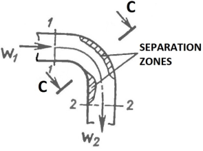
The loss coefficient ζ for the coolant flow in the heat exchanger line can be determined by analogy with the coolant flow, which is assumed to be an incompressible gas, for example, in a pipe bend (Figure 1). In Sections 1-1 and 2-2, it was assumed that the velocity profiles deviate slightly from a perfectly smooth profile.

Download: Download full-size image

Figure 1. Schematic diagram of the gas refrigerant flow curve of the heat exchange line.

We write the Bernoulli equation for such a flow of gaseous refrigerant (p0 is the flow pressure or total pressure at the stagnation point)

[1, 6, 7]

p_{1} + ρ \frac{W_{1}^{2}}{2} = p_{2} + ρ \frac{W_{2}^{2}}{2} + ζρ \frac{W_{2}^{2}}{2}

(2)

The first two terms on the left and right represent the stagnation flow pressure; therefore, the incompressible gas cooling loss coefficient ζ represents the relative percentage of the total pressure loss:

ζ = \frac{p_{01} - p_{02}}{ρ \frac{W_{2}^{2}}{2}}

(3)

Therefore, for example, it is necessary to determine the total pressure loss using experimental data, and

ρ \frac{W_{2}^{2}}{2}

. The total pressure can be determined experimentally, for example, using a total pressure sensor. If the volumetric flow rate of the refrigerant in the gas is known, the velocity W₂ can be calculated, for example, experimentally, using the relationship.G=ρW₂A₂(A is the cross-sectional area of the heat exchange tube).

For an uncompressed gaseous refrigerant in the heat exchanger, the flow rate changes in section 2-2. The loss coefficient is determined by the change in cross-sectional area A1 and A2, since the continuity equation at constant gas density - ρ₁on'₁to₁= ρ₂on'₂to₂- W stands for equality₂= 2₁· (to₁/to₂). As a result, the loss coefficient represents the relative contribution of the static pressure loss. The relationship between the resistance coefficient ζ and the Bernoulli equation for the leaking coolant flow can be obtained by equating the Bernoulli equation for the leaking flow ((p2)id is the static pressure in the 2-2 section of the leaking flow)

[1, 6, 7]

ζ = \frac{{(p_{2})}_{ид} - p_{2}}{ρ \frac{W_{2}^{2}}{2}}

(4)

The gas flow in the heat exchanger tube bend is a non-one-dimensional flow with a complex spatial structure that depends on the properties of the incoming gas coolant and the geometry of the channel. Due to inertial forces, the initial linear motion remains, the pressure increases on the outer wall of the channel and decreases on the inner wall. The velocity of the gas particles in the boundary layer is relatively small in the direction of the main flow. The pressure gradient created in the cross section causes the particles to move from the outer wall to the inner wall along the circumference of the channel, creating a compensating counter-rotation in the gas core. This leads to the formation of a secondary motion in the cross section in the form of a pair of vortices.

The main flow rate of the gas refrigerant in the pipe bend. The flow velocity in the heat exchanger channel is inversely proportional to the change in pressure: the velocity of the refrigerant outside the boundary layer decreases compared to the velocity in the section 1-1. The flow is distributed on the outer wall, and on the inner wall outside the boundary layer. With a small bend in the heat exchanger pipe, the boundary layer pressure can be almost equal to the pressure of the standing flow, and a vortex zone can form along the wall. After passing through the central section CC, a redistribution of the velocity and pressure profiles occurs, the pressure decreases from the inner wall to the outer wall, and the velocity increases. The curvature of the inner wall of the heat exchanger pipe relative to the main flow direction and the above-mentioned pressure increase contribute to the formation of a boundary layer separation zone, the thickness and length of which are significantly greater than the corresponding dimensions of the separation zone on the outer wall.

[1, 2, 4-8]

The total energy loss of the gas refrigerant flow in the flow line of the heat exchanger can be divided into friction loss and internal loss. The energy loss can be classified as follows: friction and power loss are caused by the non-uniformity of the velocity field and its subsequent smoothing. Internal loss is determined by the friction loss caused by the second flow and the loss caused by the formation of the vortex flow region. Internal loss and power loss account for most of the total energy loss.

The degree of non-uniformity of the velocity field, the size of the separation zone and the intensity of the second flow depend on the geometric parameters of the heat exchanger tube bend and the Reynolds number Re. The change of the resistance coefficient ζ in the heat exchanger tube as a function of the above-mentioned parameters can be determined, for example, using experimental data

[2, 4, 5, 8, 9]

As the pressure drop and the size of the separation zone increase, the losses increase along with the non-uniform velocity field of the incoming refrigerant. Since the movement number (M) of the refrigerant flow in the heat exchange line is low, its effect on the resistance coefficient is very small. The velocity field becomes more uniform in long pipe sections connected by bends. Since heat exchange lines can be short in practice, it is necessary to average the parameters of sections 1-1 and 2-2 to determine the resistance coefficient (ζ).

Averaging of gas coolant parameters in heat transfer: Averaging in a heat exchanger allows us to move from considering a flow with a non-uniform distribution of parameters in space to a flow with a uniform distribution of parameters along the cross-section of the heat exchanger tubes, and thus from a large number of actual flow parameter values - more precisely, from vector or scalar parameter fields - to a significantly smaller number of average flow parameters. To simplify the averaging calculation methods, a number of provisions are made that reflect the characteristics of the actual gas coolant flow in the heat exchanger tube elements. Note that: if the gas coolant flow is characterized by almost no heat exchange with the environment, then the stagnation temperature T* can be assumed to be constant at all points along the cross-section of the heat balance line. When determining the loss coefficients in the bends and branches of the heat balance line, in most cases they can be assumed to be constant along the inlet and outlet cross-sections.

The loss coefficient ζ can be related to the plus parameters at the outlet and inlet of the heat exchange line. For example, the energy loss can be defined as follows (W'₂is the plus mass flow rate of the gaseous refrigerant excluding losses at the outlet of the line)

[1, 6, 7]

l_{п} = ζρ \frac{{(W_{2}^{'})}^{2}}{2}

(5)

Therefore, when using experimental values for the resistance coefficient ζ for branched heat exchanger lines, special attention should be paid to the type of expression that determines the aforementioned coefficient.

Furthermore, when calculating the flow parameters of an incompressible gaseous coolant, taking into account hydromechanical losses in heat exchanger lines, it is not correct to use the equality of temperatures of the stagnant flow, since the relationship between T₀₁ and T₀₂ is determined by the equation of state.

To determine the loss coefficientζ for pipe branches. For the heat exchanger channels of a coolant in the form of a compressed gas, the structure of formula (3) can be used. The following expression:

ζ = \frac{p_{01} - p_{02}}{ϱ_{02} \frac{W_{2}^{2}}{2}}

(6)

establishes a relationship between the resistance coefficientsζand restoration of the total pressure σ (σ=p₀₂/p₀₁) during the flow of gaseous coolant in the pipes of heat exchangers. After the conversions, we obtain:

σ = {(1 + ζ \frac{W_{2}^{2}}{2 R T_{02}})}^{- 1}

(7)

Power loss of compressed gas the coolant flow in the heat exchanger line can be estimated using the loss coefficient ζ_сж, if work is defined as the adiabatic compression work required to reset the total pressure p₀₂ to the initial pressure p01

[1, 6, 7]

ζ_{сж} = \frac{l}{\frac{W_{1}^{2}}{2}} = \frac{{\frac{γ}{γ - 1} RT}_{02} ({(\frac{p_{01}}{p_{02}})}^{\frac{γ - 1}{γ}} - 1)}{\frac{W_{1}^{2}}{2}}

(8)

For the mathematical modeling of the flow of a gaseous coolant in the branches of heat exchanger lines, which has an acceptable degree of approximation to the actual flow and the complexity of the necessary calculations, it is therefore useful to choose a thermodynamic model of the subcritical steady flow of compressed gas.

2. Mathematical Modeling of the Flow Parameters of Gas-Formed Coolants in Branches of Heat Exchange Lines

In an energy-isolated isentropic flow, the thermodynamic parameters of the gaseous coolant are related as follows (γ is the isentropic index)

[1, 6, 7]

T_{0} = T (1 + \frac{γ - 1}{2} М^{2});

(9)

ϱ_{0} = ϱ {(1 + \frac{γ - 1}{2} М^{2})}^{\frac{1}{γ - 1}};

(10)

p_{0} = p {(1 + \frac{γ - 1}{2} М^{2})}^{\frac{γ}{γ - 1}} .

(11)

The parameters of a one-dimensional steady flow at the outlet in section 2-2 (Figure 1) of the gas dynamic device of a heat exchanger are determined when the parameters at the inlet 1-1 are known, with a known value of the total pressure recovery coefficient σ=p₀₂/p₀₁ (p₀ is the pressure of the stagnant flow or the total pressure), which is determined from the solution of a system of nonlinear equations:

\{\begin{matrix} p_{01} σ = p_{02} = p_{2} {(1 + \frac{γ - 1}{2} \frac{W_{2}^{2}}{γ R T_{2}})}^{\frac{γ}{γ - 1}}; \\ T_{01} = T_{02} = T_{2} (1 + \frac{γ - 1}{2} \frac{W_{2}^{2}}{γ R T_{2}}); \\ G = A_{2} \frac{p_{2}}{R T_{2}} W_{2} . \end{matrix}

(12)

The last system of equations can be applied to the calculation method for the steady flow of a gaseous coolant with a more complex flow structure in triple branches or T-pieces of heat exchanger lines.

The analytical solution of the specific system of equations (12) can be represented in the following form:

[\begin{matrix} p_{2} {= p_{01} σ (\frac{T_{2}}{T_{01}})}^{\frac{γ}{γ - 1}}; \\ W_{2} = \sqrt{2 R \frac{γ}{γ - 1} (T_{01} - T_{2})}; \\ A_{2} = {(\frac{T_{01}}{T_{2}})}^{\frac{γ}{γ - 1}} \frac{G T_{2}}{p_{01} σ} \sqrt{\frac{R}{2 (T_{01} - T_{2})} \frac{γ - 1}{γ}} . \end{matrix}

(13)

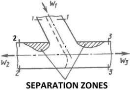
The diagram of this flow, more precisely the separation of the gaseous coolant flow in the heat exchanger piping with the parameter designations in characteristic sections, is shown in Figure 2.

Download: Download full-size image

Figure 2. Diagram of the flow of separate streams of gaseous coolant in the branch of the heat exchanger line.

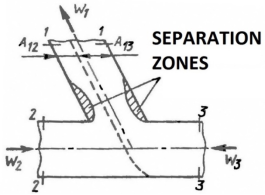
Рower lines The dashed lines in Figure 2 show the division of the flow entering the fork into two streams exiting through the branches. In Figure 3, the dashed lines correspond to the dividing lines where the streams converge.

Download: Download full-size image

Figure 3. Flow diagram when gaseous coolant flows are combined in a branch of a heat exchanger line.

Gas flow in a branched piping system of a heat exchanger is characterized by a complex spatial structure with a non-uniform distribution of parameters in sections 2-2 and 3-3.

It is assumed that the flows of the gaseous coolant do not influence each other. The values of the parameters in section 1-1 and the recovery coefficients σ1 and σ2 are known; the pressures in sections 2-2 and 3-3 are assumed to be practically equal. These assumptions allow us to formulate a system of nonlinear equations for determining the parameters of the gaseous refrigerant in sections 2-2 and 3-3 above:

\{\begin{matrix} p_{01} σ_{1} = p_{02} = p_{2} {(1 + \frac{γ - 1}{2} \frac{W_{2}^{2}}{γ R T_{2}})}^{\frac{γ}{γ - 1}}; \\ p_{01} σ_{2} = p_{03} = p_{3} {(1 + \frac{γ - 1}{2} \frac{W_{3}^{2}}{γ R T_{3}})}^{\frac{γ}{γ - 1}}; \\ T_{01} = T_{02} = T_{2} (1 + \frac{γ - 1}{2} \frac{W_{2}^{2}}{γ R T_{2}}); \\ T_{01} = T_{03} = T_{3} (1 + \frac{γ - 1}{2} \frac{W_{3}^{2}}{γ R T_{3}}); \\ G = A_{2} \frac{p_{2}}{R T_{2}} W_{2} + A_{3} \frac{p_{3}}{R T_{3}} W_{3}; \\ p_{2} = p_{3} . \end{matrix}

(14)

For the considered model of one-dimensional steady flow in a branched heat exchanger line, the structure and the parameters to be determined must be defined before solving the associated system of equations. Since the flow in heat exchanger lines is subcritical, the pressure values in sections 2-2 and 3-3, as well as two parameters in section 1-1, must be determined. This choice of independent parameters for the state of the gaseous coolant in the branched sections corresponds to the flow patterns described above.

In a one-dimensional model, the flow parameters of the gaseous coolant must satisfy the condition of equalization after flow merging. It is assumed that no heat or mass transfer processes occur between the gas flows passing through the different regions A₁₂ and A₁₃ (A₁ = A₁₂ + A₁₃) in section 1-1 (Figure 3); therefore, they have different densities and velocities, but the same pressure.

3. Analytical Solutions for the Problem of Gas Shark Coolant Flow in Branches of Heat Exchange Excludes

The flow of gaseous coolant in the branches of heat pipes: The exchange of gases in these devices is accompanied by turbulence and the formation of separation zones, which in turn leads to significant losses of mechanical energy.

Qualitative and quantitative: The estimation of losses and the flow structure in steady flows in the branching of heat exchanger lines is usually based on an experiment.

In the vast majority of cases, the parameters for steady-state gas flows in heat exchanger lines are investigated, since the main flow regime under these conditions is turbulent-steady-state.

When calculating flow parameters in heat exchanger lines, additional assumptions should be taken into account, such as the constancy of the channel shape and the separation or merging of gas flows (Figures 2, 3).

In this case, we consider the method for calculating the parameters in the branches of heat exchanger piping, restricting ourselves to the task of determining the boundary conditions of the differential problem of non-stationary one-dimensional flows in straight sections of piping.

The boundary conditions are defined as follows. For open boundaries, the number of defined boundary conditions corresponds to the number of characteristic curves emanating from the boundary, while the boundary conditions for the incoming characteristic curves are determined by solving the differential equation problem. Assuming that the required parameters of the gaseous coolant in the cross-section of a heat exchanger line that branches near a nozzle or vessel are known, and based on the postulated determinations for defining the boundary conditions, the system of initial equations for calculating possible cases of gaseous coolant flow in the branch can thus be derived

[1, 6, 7]

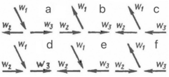
The following cases of flow separation and merging in a triple branch or T-piece are possible in heat exchanger lines. Possible: (Figure 4). For simplicity, the cross-sections are labeled Figure 2 and Figure 3, respectively. This study shows the assignment of boundary conditions that apply to all cases and implements analytical solutions only for the most important cases of gaseous coolant flows in the branches of heat exchangers.

Download: Download full-size image

Figure 4. Typical flow diagrams of gaseous coolant flows in the branches of heat exchanger lines.

Around theTo separate flows in the piping of a heat exchanger (Figure 4a) In section 3-3, two boundary conditions must be specified, since two characteristics deviate from this boundary; in section 2-2, the positions of the characteristics at pressure p₂or velocity W₂ and temperature T₂ must be specified, since the positions of the characteristics are similar to those in section 3-3.

The main system of equations for this case of separation or merging of flows in the piping of a heat exchanger is the system of equations (13).

Cases of flow separation in the piping of a heat exchangerSince Figures 4b and 4c are symmetrical, we can restrict ourselves to the first case. In Section 2-2, a boundary condition must be specified, as only one property deviates from it: equality of the outlet pressures: p₁ = p₃. In Section 1-1, the parameters sought are temperature T₁ and velocity W₂ or pressure p₁.

Now we will consider the method for defining boundary conditions for combining flows in the piping of heat exchangers.

The algorithms for calculating flow confluence in heat exchanger lines for the cases shown in Figures 4d and 4e are similar; therefore, we consider only the first case. For flow confluence in the heat exchanger line according to Figure 4e, one boundary condition must be defined in section 2-2 and two in section 3-3. It is assumed that the coolant flows entering through sections 1-1 and 2-2 do not mix. Therefore, the required parameters are the cross-sectional areas A₃₁ and A₃₂ (A₃₁ + A₃₂ = A₃), which correspond to the gaseous coolant flows exiting through section 3-3.

It is assumed that the temperatures T₃₁ and T₃₂ and the velocities W₃₁ and W₃₂ of the outflowing liquids are different, that the pressure is the same in section 3-3 and that p₂=p₁ also applies.

Taking into account the above assumptions, the main system (13) yields the system of output equations for calculating the flow rate of gaseous coolant in the pipeline of a heat exchanger during flow separation (Figure 4a):

\{\begin{matrix} p_{01} σ_{1} = p_{3} {(1 + \frac{γ - 1}{2} \frac{W_{31}^{2}}{γ R T_{31}})}^{\frac{γ}{γ - 1}}; \\ p_{02} σ_{2} = p_{3} {(1 + \frac{γ - 1}{2} \frac{W_{32}^{2}}{γ R T_{32}})}^{\frac{γ}{γ - 1}}; \\ T_{01} = T_{31} (1 + \frac{γ - 1}{2} \frac{W_{31}^{2}}{γ R T_{31}}); \\ T_{02} = T_{32} (1 + \frac{γ - 1}{2} \frac{W_{32}^{2}}{γ R T_{32}}); \\ G_{1} = A_{31} \frac{p_{3}}{R T_{31}} W_{31}; \\ A_{2} \frac{p_{2}}{R T_{2}} W_{2} = (A_{3} {- A}_{31}) \frac{p_{3}}{R T_{32}} W_{32} . \end{matrix}

(15)

PressureR₂is known as a boundary condition in Section 2-2; the flow rate G1 of the gaseous coolant through Section 1-1 is also known.

The unknown parameters are the velocities W₂, W₃₁, W₃₂ and the temperatures T₃₁, T₃₂, as well as the cross-sectional area A₃₁. This results in a system of six nonlinear equations with six unknowns. This system of equations can be solved analytically, although it was previously determined that it can only be solved numerically

[6]

. System (14) has four analytical solutions.

The solution to the system of equations yields 4 roots, of which only one has a physical meaning and, after simplifications, takes the following form:

[\begin{matrix} W_{2} = \sqrt{1 - {(\frac{p_{02}}{p_{3}} σ_{2})}^{\frac{1 - γ}{γ}}} \sqrt{R} \frac{{(p_{02} σ_{2})}^{\frac{γ - 1}{γ}} T_{2}}{A_{2} p_{2} \sqrt{T_{02}}} (A_{3} \sqrt{2 \frac{γ}{γ - 1}} p_{3}^{\frac{1}{γ}} - \frac{\sqrt{R} {(p_{01} σ_{1})}^{\frac{1 - γ}{γ}} \sqrt{T_{01}} G_{1}}{\sqrt{1 - {(\frac{p_{01}}{p_{3}} σ_{1})}^{\frac{1 - γ}{γ}}}}); \\ W_{31} = \sqrt{\frac{2 γ}{1 - γ} R T_{01} ({(\frac{p_{01}}{p_{3}} σ_{1})}^{\frac{1 - γ}{γ}} - 1)}; \\ W_{32} = \sqrt{\frac{2 γ}{1 - γ} R T_{02} ({(\frac{p_{02}}{p_{3}} σ_{2})}^{\frac{1 - γ}{γ}} - 1)}; \\ T_{31} = T_{01} {(\frac{p_{01}}{p_{3}} σ_{1})}^{\frac{1 - γ}{γ}}; \\ T_{32} = T_{02} {(\frac{p_{02}}{p_{3}} σ_{2})}^{\frac{1 - γ}{γ}}; \\ A_{31} = \frac{G_{1}}{p_{3}} {(\frac{p_{01}}{p_{3}} σ_{1})}^{\frac{1 - γ}{γ}} \frac{\sqrt{\frac{γ - 1}{2 γ} R T_{01}}}{\sqrt{1 - {(\frac{p_{01}}{p_{3}} σ_{1})}^{\frac{1 - γ}{γ}}}} . \end{matrix}

(16)

NextLet's consider. Algorithm for calculating the merging of flows in heat exchanger lines for the cases shown in Figure 4f.

In the case of combining flows in the heat exchanger line, as shown in Figure 4f, only one boundary condition is determined in sections 2-2 and 3-3, since the main condition for this case of combining flows is the condition of equality of pressures p₂=p₃, which is specified as a boundary condition.

In this case, an unknown parameter can be specified - the pressure p₂. For section 1-1, the unknown parameters are the velocities, temperatures, and cross-sectional areas: W₁₂, W₁₃, T₁₂, T₁₃, A₁₂, A₁₃, where (A₁=A₁₂+A₁₃).

Taking into account the above assumptions, the main system (13) yields the system of output equations for calculating the flow rate of the gaseous coolant in the pipeline of a heat exchanger when the flows are combined (Figure 4f):

\{\begin{matrix} p_{02} σ_{2} = p_{1} {(1 + \frac{γ - 1}{2} \frac{W_{12}^{2}}{γ R T_{12}})}^{\frac{γ}{γ - 1}}; \\ p_{03} σ_{3} = p_{1} {(1 + \frac{γ - 1}{2} \frac{W_{13}^{2}}{γ R T_{13}})}^{\frac{γ}{γ - 1}}; \\ T_{02} = T_{12} (1 + \frac{γ - 1}{2} \frac{W_{12}^{2}}{γ R T_{12}}); \\ T_{03} = T_{13} (1 + \frac{γ - 1}{2} \frac{W_{13}^{2}}{γ R T_{13}}); \\ A_{2} \frac{p_{2}}{R T_{2}} W_{2} = A_{12} \frac{p_{1}}{R T_{12}} W_{12}; \\ A_{3} \frac{p_{2}}{R T_{3}} W_{3} = (A_{1} {- A}_{12}) \frac{p_{1}}{R T_{13}} W_{13} . \end{matrix}

(17)

Here too, we have a system of six linear and nonlinear equations with six unknowns. This system of equations can be solved analytically, although it was previously established that it can only be solved numerically

[6]

. System (17) has four analytical solutions. The solution of the system yields four roots, only one of which has a physical meaning and, after simplification, takes the following form:

[\begin{matrix} p_{2} = \sqrt{\frac{2 γ}{1 - γ} R} \frac{A_{1} p_{1} \sqrt{({1 - (\frac{p_{02}}{p_{1}} σ_{2})}^{\frac{1 - γ}{γ}}) ({1 - (\frac{p_{03}}{p_{1}} σ_{3})}^{\frac{1 - γ}{γ}})}}{{A_{3} (\frac{p_{03}}{p_{1}} σ_{3})}^{\frac{1 - γ}{γ}} W_{3} \frac{\sqrt{T_{03}}}{T_{3}} \sqrt{{1 - (\frac{p_{02}}{p_{1}} σ_{2})}^{\frac{1 - γ}{γ}}} + {A_{2} (\frac{p_{02}}{p_{1}} σ_{2})}^{\frac{1 - γ}{γ}} W_{2} \frac{\sqrt{T_{02}}}{T_{2}} \sqrt{{1 - (\frac{p_{03}}{p_{1}} σ_{3})}^{\frac{1 - γ}{γ}}}}; \\ W_{12} = \sqrt{\frac{2 γ}{1 - γ} R T_{02} ({(\frac{p_{02}}{p_{1}} σ_{2})}^{\frac{1 - γ}{γ}} - 1)}; \\ W_{13} = \sqrt{\frac{2 γ}{1 - γ} R T_{03} ({(\frac{p_{03}}{p_{1}} σ_{3})}^{\frac{1 - γ}{γ}} - 1)}; \\ T_{12} = T_{02} {(\frac{p_{02}}{p_{1}} σ_{2})}^{\frac{1 - γ}{γ}}; \\ T_{13} = T_{03} {(\frac{p_{03}}{p_{1}} σ_{3})}^{\frac{1 - γ}{γ}}; \\ A_{12} = \frac{A_{1} \sqrt{{1 - (\frac{p_{03}}{p_{1}} σ_{3})}^{\frac{1 - γ}{γ}}}}{\sqrt{{1 - (\frac{p_{03}}{p_{1}} σ_{3})}^{\frac{1 - γ}{γ}}} + \frac{A_{3}}{A_{2}} {(\frac{σ_{2}}{σ_{3}})}^{\frac{γ - 1}{γ}} {(\frac{p_{02}}{p_{03}})}^{\frac{γ - 1}{γ}} \frac{W_{3}}{W_{2}} \frac{T_{2}}{T_{3}} \sqrt{\frac{T_{03}}{T_{02}}} \sqrt{{1 - (\frac{p_{02}}{p_{1}} σ_{2})}^{\frac{1 - γ}{γ}}}} . \end{matrix}

(18)

Solutions (15) and (17) were verified numerically and using the tools of symbolic computational mathematics

[10-12]

With appropriately similar definition of the boundary conditions, the problem of determining the parameters of a gaseous coolant in a heat exchanger pipe bend can be solved analytically much more easily than in a T-piece

[13]	Lobanov I. E. Analytical Solution of the Problem of Stationary Subcritical Flow of a Gaseous Heat Carrier in the Branches of Heat Exchanger Pipes // Actual Problems of Cosmonautics: Proceedings of the XLII Academic Readings on Cosmonautics Dedicated to the Memory of Academician S. P. Korolev and Other Outstanding Russian Scientists and Pioneers of Space Exploration. Moscow, January 23-26, 2018. Moscow: Bauman Moscow State Technical University, 2018. pp. 132-133.
[14]	Lobanov I. E. Theoretical accurate analytical solution to the problem of mathematical modeling of stationary subcritical flow of a gaseous coolant in the ramifications of pipelines of heat exchangers // Web portal of the professional network pedagogical community "Ped-library.ru ". 2018. Access mode: https://ped-library.ru/1545740571 View Article
[15]	Lobanov I. E. A theoretical accurate analytical solution to the problem of mathematical modeling of stationary subcritical flow of a gaseous coolant in the branches of pipelines of heat exchangers // Innovative approaches in industries and spheres. 2019. Vol. 4. Issue 2 (February, 2019). Access mode: http://inf16.ru/vypusk-2-fevral-2019 View Article
[16]	Lobanov I. E. Theoretical Solution of the Problem for Subcritical Stationary Flow of a Gaseous Heat Carrier in Pipeline Branches // All-Russian Scientific and Practical Conference "Modern Science and Education: Current Problems of Theory and Practice". Materials of the All-Russian Scientific and Practical Conference. Cheboksary: Non-State Educational Institution of Additional Professional Education "Expert and Methodological Center", 2019. Pp. 9-29.
[17]	Lobanov I. E. Theoretical Analytical Solution of the Problem of Stationary Subcritical Flow of a Gaseous Heat Carrier in the Branching of Heat Exchanger Pipes // Bulletin of Bryansk State Technical University. 2019. № 9. P. 25-35. https://doi.org/10.30987/article_5d9317b27868a4.78923465 View Article
[18]	Lobanov I. E. Analytical Solution of the Problem of Stationary Subcritical Flow of a Gaseous Heat Carrier in the Branches of Pipelines of Heat Exchangers // Acta Scientific Computer Sciences. 2020. Volume 2. Issue 9. P. 29-30.

[13-18]

The presented analytical solutions for a specific problem of combining gaseous coolant flows in heat exchanger lines justify the derivation of similar analytical solutions for the separation of flows

[19]

The following results were obtained in this study: analytical solutions for the problem of flow in branches of gaseous coolant flows in heat exchanger lines, whereas previously only numerical solutions existed for this problem

[20-22]

4. Result

In this work, the choice of a theoretical model for the mathematical modeling of the flow of a gaseous coolant in the branches of heat exchanger lines was justified, which has an acceptable degree of closeness to the actual flow and to the complexity of the necessary calculations - a thermodynamic model of the subcritical steady flow of compressed gas.

5. Discussion

Analytical solutions have been found for the problem of flow in branches of gaseous coolant flows in heat exchanger lines, whereas previously only numerical solutions to this problem had been found.

Abbreviations

G	Mass Consumption, kg/c
W	Speed, m/s
ρ	Density, kg/m³
µ	Expense Ratio
L	Work, J
l	Work Per Unit of Time, J/s
ζ	Loss Ratio
p	Pressure, P
A	Cross-Sectional Area, m²
γ	Isentropy Index
σ	Full Pressure Recovery Coefficient
Re	Reynolds Number
M	Mach Number
R	Gas Constant, J/(kg·К)
T	Temperature, K

Author Contributions

Lobanov Igor Evgenievich: Conceptualization, Data curation, Formal Analysis, Methodology, Software, Visualization

Conflicts of Interest

The author declares no conflicts of interest.

References

[1]	Abramovich G. N. Applied Gas Dynamics. M.: Nauka, 1976. 888 pp.
[2]	Altshul A. D. Hydraulic Resistances. M.: Nedra, 1982. 224 pp.
[3]	Idelchik I. E. Aerohydrodynamics of technological devices. (Supply, removal and distribution) flow From Section Devices). M.: Mechanical engineering, 1983. 351 pages.
[4]	Idelchik I. E. Handbook of Hydraulic Resistance. M.: Mashinostroenie, 1975. 427 pp.
[5]	Idelchik I. E. Handbook of Hydraulic Resistance / Ed. MO Steinberg. M.: Mashinostroenie, 1992. 672 pp.
[6]	Kruglov M. G., Mednov A. A. Gas Dynamics of Combined Internal Combustion Engines. M.: Mashinostroenie, 1988. 360 pp.
[7]	Loitsyansky L. G. Mechanics of Liquids and Gases. M.: Nauka, 1987. 840 pp.
[8]	Handbook of Calculations for Hydraulic and Ventilation Systems. / Ed. A. S. Juriev. St. Petersburg: ANO NPO "Peace and Family", 2001. 1154 pp.
[9]	Shevelev F. A. Tables for the hydraulic calculation of water and steam pipes made of steel, cast iron, asbestos cement, plastic and glass. M.: Stroyizdat, 1973. 112 pp.
[10]	Lobanov I. E. Analytical Solution of the Problem of Stationary Subcritical Flow of a Gaseous Heat Carrier in the Branches of Heat Exchanger Tubing: Formulation of the Research Problem // Electronic Scientific Journal "Industry-Specific Aspects of Technical Sciences". 2016. Issue 1 (49). January-February. Pp. 12-16.
[11]	Lobanov I. E. On the Solution of the Problem of Stationary Subcritical Flow of a Gaseous Heat Carrier in the Branches of Heat Exchanger Pipelines // Electronic Periodical Peer-Reviewed Scientific Journal "SCI-ARTICLE. RU". 2016. No. 29 (January). Pp. 141-150.
[12]	Lobanov I. E. An accurate theoretical analytical solution to the problem of stationary subcritical flow of a gaseous heat carrier in the branches of pipelines of heat exchange devices and heat exchange units // Electronic periodical peer-reviewed scientific journal "SCI-ARTICLE. RU". 2017. № 42 (February). Pp. 143-152.
[13]	Lobanov I. E. Analytical Solution of the Problem of Stationary Subcritical Flow of a Gaseous Heat Carrier in the Branches of Heat Exchanger Pipes // Actual Problems of Cosmonautics: Proceedings of the XLII Academic Readings on Cosmonautics Dedicated to the Memory of Academician S. P. Korolev and Other Outstanding Russian Scientists and Pioneers of Space Exploration. Moscow, January 23-26, 2018. Moscow: Bauman Moscow State Technical University, 2018. pp. 132-133.
[14]	Lobanov I. E. Theoretical accurate analytical solution to the problem of mathematical modeling of stationary subcritical flow of a gaseous coolant in the ramifications of pipelines of heat exchangers // Web portal of the professional network pedagogical community "Ped-library.ru ". 2018. Access mode: https://ped-library.ru/1545740571
[15]	Lobanov I. E. A theoretical accurate analytical solution to the problem of mathematical modeling of stationary subcritical flow of a gaseous coolant in the branches of pipelines of heat exchangers // Innovative approaches in industries and spheres. 2019. Vol. 4. Issue 2 (February, 2019). Access mode: http://inf16.ru/vypusk-2-fevral-2019
[16]	Lobanov I. E. Theoretical Solution of the Problem for Subcritical Stationary Flow of a Gaseous Heat Carrier in Pipeline Branches // All-Russian Scientific and Practical Conference "Modern Science and Education: Current Problems of Theory and Practice". Materials of the All-Russian Scientific and Practical Conference. Cheboksary: Non-State Educational Institution of Additional Professional Education "Expert and Methodological Center", 2019. Pp. 9-29.
[17]	Lobanov I. E. Theoretical Analytical Solution of the Problem of Stationary Subcritical Flow of a Gaseous Heat Carrier in the Branching of Heat Exchanger Pipes // Bulletin of Bryansk State Technical University. 2019. № 9. P. 25-35. https://doi.org/10.30987/article_5d9317b27868a4.78923465
[18]	Lobanov I. E. Analytical Solution of the Problem of Stationary Subcritical Flow of a Gaseous Heat Carrier in the Branches of Pipelines of Heat Exchangers // Acta Scientific Computer Sciences. 2020. Volume 2. Issue 9. P. 29-30.
[19]	Lobanov I. E. Theoretical Exact Analytical Solution of the Problem of Mathematical Modeling of the Stationary of the Decritical Flow of a Gaseous Heat Carrier in Branches of Heat Exchange Pipelines Apparatus // Global Journal of Astronomy and Applied Physics. 2021. Volume: 3: 1004. Issue: 1. P. 1-9.
[20]	Lobanov I. E. Accurate analytical solution of the problem of stationary subcritical flow of gaseous coolant in the branches of the pipeline of the heat exchange apparatus // Network publication "International Pedagogical Portal "Sunlight"". 2021. Access mode: https://solncesvet.ru/opublikovannyie-materialyi/tochnoe-analiticheskoe-reshenie-zadachi-.5779692
[21]	Lobanov I. E. Analytical Solution of the Stationary Subcritical Flow of a Gaseous Coolant in the Branches of the Heat Exchange Pipelines of the Apparatus // International Journal of Healthcare Systems Engineering. 2021. Volume 3. Issue 7. P. 1-10. https://doi.org/10.35840/2633-8939/7207
[22]	Lobanov I. E. Mathematical Numerical And Analytical Solutions To The Problem Of Longitudinal Velocity Distribution In A Single Row System Of Impact Plane Parallel Jets Flowing On A Plane Surface With Allow-ance For Losses In Nozzles And Friction // Current Research in Statistics & Mathematics. 2025. Volume 4. Issue 1. Pp. 1-8.

Cite This Article

Plain Text BibTeX RIS

APA Style

Evgenievich, L. I. (2026). Theoretical-analytical Solution to the Problem of Steady Subcritical Flow of Gaseous Coolant in Branches of Pipelines of Heat Exchange Units. International Journal of Mechanical Engineering and Applications, 14(5), 132-140. https://doi.org/10.11648/j.ijmea.20261405.15

Copy | Download

ACS Style

Evgenievich, L. I. Theoretical-analytical Solution to the Problem of Steady Subcritical Flow of Gaseous Coolant in Branches of Pipelines of Heat Exchange Units. Int. J. Mech. Eng. Appl. 2026, 14(5), 132-140. doi: 10.11648/j.ijmea.20261405.15

Copy | Download

AMA Style

Evgenievich LI. Theoretical-analytical Solution to the Problem of Steady Subcritical Flow of Gaseous Coolant in Branches of Pipelines of Heat Exchange Units. Int J Mech Eng Appl. 2026;14(5):132-140. doi: 10.11648/j.ijmea.20261405.15

Copy | Download

@article{10.11648/j.ijmea.20261405.15,
  author = {Lobanov Igor Evgenievich},
  title = {Theoretical-analytical Solution to the Problem of Steady Subcritical Flow of Gaseous Coolant in Branches of Pipelines of Heat Exchange Units},
  journal = {International Journal of Mechanical Engineering and Applications},
  volume = {14},
  number = {5},
  pages = {132-140},
  doi = {10.11648/j.ijmea.20261405.15},
  url = {https://doi.org/10.11648/j.ijmea.20261405.15},
  eprint = {https://article.sciencepublishinggroup.com/pdf/10.11648.j.ijmea.20261405.15},
  abstract = {The study provides analytical solutions to the problem of determining the flow parameters at the branch points of the coolant flow in a heat exchanger line. Previously, only numerical solutions to the problem were considered. In this work, the choice of a theoretical model for mathematical modeling of the flow of a refrigerant in a gas in the heat exchange line branch is justified, which shows an acceptable level of approximation to the real flow and the required computational complexity: a thermodynamic model of a stable subcritical flow of compressed gas. With the appropriate analog definition of boundary conditions, the problem of determining the parameters of the gas refrigerant in the heat exchanger tube bend can be solved analytically much easier than for a T-shaped connector. The analytical solutions presented for the specific problem of combining the gas refrigerant flow in the heat exchanger line serve as a basis for performing similar analytical solutions for the separation of the flows. The following results were obtained in this study: Analytical solutions for the dual flow problem of the gas refrigerant flow in the heat exchanger line, previously only numerical solutions were available for this problem.},
 year = {2026}
}

Copy | Download

TY  - JOUR
T1  - Theoretical-analytical Solution to the Problem of Steady Subcritical Flow of Gaseous Coolant in Branches of Pipelines of Heat Exchange Units
AU  - Lobanov Igor Evgenievich
Y1  - 2026/10/26
PY  - 2026
N1  - https://doi.org/10.11648/j.ijmea.20261405.15
DO  - 10.11648/j.ijmea.20261405.15
T2  - International Journal of Mechanical Engineering and Applications
JF  - International Journal of Mechanical Engineering and Applications
JO  - International Journal of Mechanical Engineering and Applications
SP  - 132
EP  - 140
PB  - Science Publishing Group
SN  - 2330-0248
UR  - https://doi.org/10.11648/j.ijmea.20261405.15
AB  - The study provides analytical solutions to the problem of determining the flow parameters at the branch points of the coolant flow in a heat exchanger line. Previously, only numerical solutions to the problem were considered. In this work, the choice of a theoretical model for mathematical modeling of the flow of a refrigerant in a gas in the heat exchange line branch is justified, which shows an acceptable level of approximation to the real flow and the required computational complexity: a thermodynamic model of a stable subcritical flow of compressed gas. With the appropriate analog definition of boundary conditions, the problem of determining the parameters of the gas refrigerant in the heat exchanger tube bend can be solved analytically much easier than for a T-shaped connector. The analytical solutions presented for the specific problem of combining the gas refrigerant flow in the heat exchanger line serve as a basis for performing similar analytical solutions for the separation of the flows. The following results were obtained in this study: Analytical solutions for the dual flow problem of the gas refrigerant flow in the heat exchanger line, previously only numerical solutions were available for this problem.
VL  - 14
IS  - 5
ER  -

Copy | Download

Author Information

Lobanov Igor Evgenievich

Department of Engineering and Technology, Technological University named after A. A. Leonov, Korolyov, Russia

Contact Email

http://orcid.org/0000-0001-8421-0248

Download PDF

Submit an Article

Plain Text BibTeX RIS

APA Style

Evgenievich, L. I. (2026). Theoretical-analytical Solution to the Problem of Steady Subcritical Flow of Gaseous Coolant in Branches of Pipelines of Heat Exchange Units. International Journal of Mechanical Engineering and Applications, 14(5), 132-140. https://doi.org/10.11648/j.ijmea.20261405.15

Copy | Download

ACS Style

Evgenievich, L. I. Theoretical-analytical Solution to the Problem of Steady Subcritical Flow of Gaseous Coolant in Branches of Pipelines of Heat Exchange Units. Int. J. Mech. Eng. Appl. 2026, 14(5), 132-140. doi: 10.11648/j.ijmea.20261405.15

Copy | Download

AMA Style

Evgenievich LI. Theoretical-analytical Solution to the Problem of Steady Subcritical Flow of Gaseous Coolant in Branches of Pipelines of Heat Exchange Units. Int J Mech Eng Appl. 2026;14(5):132-140. doi: 10.11648/j.ijmea.20261405.15

Copy | Download

@article{10.11648/j.ijmea.20261405.15,
  author = {Lobanov Igor Evgenievich},
  title = {Theoretical-analytical Solution to the Problem of Steady Subcritical Flow of Gaseous Coolant in Branches of Pipelines of Heat Exchange Units},
  journal = {International Journal of Mechanical Engineering and Applications},
  volume = {14},
  number = {5},
  pages = {132-140},
  doi = {10.11648/j.ijmea.20261405.15},
  url = {https://doi.org/10.11648/j.ijmea.20261405.15},
  eprint = {https://article.sciencepublishinggroup.com/pdf/10.11648.j.ijmea.20261405.15},
  abstract = {The study provides analytical solutions to the problem of determining the flow parameters at the branch points of the coolant flow in a heat exchanger line. Previously, only numerical solutions to the problem were considered. In this work, the choice of a theoretical model for mathematical modeling of the flow of a refrigerant in a gas in the heat exchange line branch is justified, which shows an acceptable level of approximation to the real flow and the required computational complexity: a thermodynamic model of a stable subcritical flow of compressed gas. With the appropriate analog definition of boundary conditions, the problem of determining the parameters of the gas refrigerant in the heat exchanger tube bend can be solved analytically much easier than for a T-shaped connector. The analytical solutions presented for the specific problem of combining the gas refrigerant flow in the heat exchanger line serve as a basis for performing similar analytical solutions for the separation of the flows. The following results were obtained in this study: Analytical solutions for the dual flow problem of the gas refrigerant flow in the heat exchanger line, previously only numerical solutions were available for this problem.},
 year = {2026}
}

Copy | Download

TY  - JOUR
T1  - Theoretical-analytical Solution to the Problem of Steady Subcritical Flow of Gaseous Coolant in Branches of Pipelines of Heat Exchange Units
AU  - Lobanov Igor Evgenievich
Y1  - 2026/10/26
PY  - 2026
N1  - https://doi.org/10.11648/j.ijmea.20261405.15
DO  - 10.11648/j.ijmea.20261405.15
T2  - International Journal of Mechanical Engineering and Applications
JF  - International Journal of Mechanical Engineering and Applications
JO  - International Journal of Mechanical Engineering and Applications
SP  - 132
EP  - 140
PB  - Science Publishing Group
SN  - 2330-0248
UR  - https://doi.org/10.11648/j.ijmea.20261405.15
AB  - The study provides analytical solutions to the problem of determining the flow parameters at the branch points of the coolant flow in a heat exchanger line. Previously, only numerical solutions to the problem were considered. In this work, the choice of a theoretical model for mathematical modeling of the flow of a refrigerant in a gas in the heat exchange line branch is justified, which shows an acceptable level of approximation to the real flow and the required computational complexity: a thermodynamic model of a stable subcritical flow of compressed gas. With the appropriate analog definition of boundary conditions, the problem of determining the parameters of the gas refrigerant in the heat exchanger tube bend can be solved analytically much easier than for a T-shaped connector. The analytical solutions presented for the specific problem of combining the gas refrigerant flow in the heat exchanger line serve as a basis for performing similar analytical solutions for the separation of the flows. The following results were obtained in this study: Analytical solutions for the dual flow problem of the gas refrigerant flow in the heat exchanger line, previously only numerical solutions were available for this problem.
VL  - 14
IS  - 5
ER  -

Copy | Download