The structural integrity of welded joints are critical factors that influence the overall safety and durability of various engineering structures, especially in the fields of construction, automotive, and pipeline industries.. This research systematically investigate the effects and interactions of welding parameters such as welding current, welding voltage, gas flow rate and welding speed for enhanced structural integrity of mild-steel SKTM13A pipe butt joints. Central Composite Design (CCD) based Response Surface Methodology (RSM) was used to investigate and optimized these Tungsten Inert Gas (TIG) welding process dependent variables to minimize responses such as residual stress, distortion in weld-ment, heat flux, and maximize Peak Temperature, tensile strength of the welded joints. The results indicated model F-values of 29.81 at a P-value of <0.0001 for the tensile strength explained the significance of the employed model. Optimal tensile strength of 308.56Mpa, minimum distortion in weldment of 0.2, Peak Temperature of 1518.45°C, residual stress of 282.724Mpa and heat flux of 1500.26Kw/min were achieved at a welding current of 140A, welding voltage 24V, gas flow rate 12lit/min and welding speed of 150 cm/min. Overall, these statistics suggest that the regression model for the desired responses are robust and adequately captures the relationship with the predictor variables. In conclusion, this research has provided valuable insights into the optimization of welding parameters using Response Surface Methodology (RSM) that can be effectively apply to drive innovation and competitiveness in the welding industry.
| Published in | International Journal of Mechanical Engineering and Applications (Volume 13, Issue 1) |
| DOI | 10.11648/j.ijmea.20251301.12 |
| Page(s) | 27-52 |
| Creative Commons |
This is an Open Access article, distributed under the terms of the Creative Commons Attribution 4.0 International License (http://creativecommons.org/licenses/by/4.0/), which permits unrestricted use, distribution and reproduction in any medium or format, provided the original work is properly cited. |
| Copyright |
Copyright © The Author(s), 2025. Published by Science Publishing Group |
Analysis, Optimization, Parametric, Structural Integrity, TIG, Pipe
Alloys | % | C | Cu | Fe | Mn | N | P | S | |
|---|---|---|---|---|---|---|---|---|---|
STKM13A | Max | 0.15 | 0.4 | 98.293 | 1.1 | .01 | 0.02 | 0.027 | |
Alloys | % | C | Fe | Mn | Al | Mo | Ni | Si | Ti |
G2Si1 electrode | Max | 0.1 | 97.68 | 1.1 | 0.02 | 0.15 | 0.15 | 0.65 | 0.15 |
Parameters | Unit | Symbol | Coded value Low (-1) | Coded value High (+1) |
|---|---|---|---|---|
Current | Amp | A | 140 | 160 |
Voltage | Volt | V | 20 | 24 |
Welding speed | cm/min | S | 150 | 170 |
Gas flow rate | Lit/min | F | 12 | 14 |
Std | Run | Factor 1 | Factor 2 | Factor 3 | Factor 4 | Response 1 | Response 2 | Response 3 | Response 4 | Response 5 |
|---|---|---|---|---|---|---|---|---|---|---|
A: Current | B: Voltage | C: Weld Speed | D: Gas Flow Rate | Temperature Distribution | Residual Stress | Distortion in Weldment | Heat Flux | Tensile Strength | ||
A | V | cm/min | Lit/min | °C | MPa | mm | KW/m2 | MPa | ||
15 | 1 | 140 | 24 | 170 | 14 | 1520.04 | 284.147 | 0.21 | 674.06 | 287.19 |
2 | 2 | 160 | 20 | 150 | 12 | 1519.66 | 266.105 | 0.22 | 873.61 | 271.96 |
16 | 3 | 160 | 24 | 170 | 14 | 1519.86 | 258.797 | 0.22 | 769.4 | 274.37 |
26 | 4 | 150 | 22 | 160 | 13 | 1519.88 | 259.18 | 0.22 | 760.34 | 281.32 |
5 | 5 | 140 | 24 | 150 | 12 | 1518.45 | 282.724 | 0.2 | 1500.26 | 308.56 |
21 | 6 | 150 | 18 | 160 | 13 | 1519.8 | 243.024 | 0.25 | 800.8 | 293.371 |
23 | 7 | 150 | 22 | 140 | 13 | 1519.87 | 259.431 | 0.22 | 760.94 | 266.998 |
8 | 8 | 160 | 24 | 150 | 14 | 1519.86 | 259.79 | 0.22 | 769.4 | 277.705 |
22 | 9 | 150 | 26 | 160 | 13 | 1520.19 | 279.801 | 0.25 | 596.76 | 307.593 |
11 | 10 | 140 | 20 | 170 | 14 | 1519.64 | 255.67 | 0.22 | 882.22 | 286.857 |
13 | 11 | 140 | 24 | 170 | 12 | 1518.3 | 292.48 | 0.19 | 1577.54 | 304.463 |
20 | 12 | 150 | 22 | 160 | 15 | 1517.14 | 258.65 | 0.19 | 2179.4 | 294.781 |
10 | 13 | 160 | 20 | 170 | 12 | 1519.66 | 257.1 | 0.22 | 873.61 | 281.838 |
18 | 14 | 170 | 22 | 160 | 13 | 1519.7 | 253.52 | 0.22 | 853.87 | 269.128 |
17 | 15 | 130 | 22 | 160 | 13 | 1520.06 | 286.11 | 0.2 | 664.59 | 290.016 |
28 | 16 | 150 | 22 | 160 | 13 | 1519.23 | 259.18 | 0.22 | 1093.67 | 281.32 |
27 | 17 | 150 | 22 | 160 | 13 | 1519.23 | 259.18 | 0.22 | 1093.67 | 281.32 |
24 | 18 | 150 | 22 | 180 | 13 | 1519.8 | 259.18 | 0.22 | 800.53 | 281.32 |
19 | 19 | 150 | 22 | 160 | 11 | 1518.27 | 287.97 | 0.17 | 1593.36 | 305.61 |
4 | 20 | 160 | 20 | 150 | 14 | 1517.53 | 249.37 | 0.23 | 1976.99 | 268.224 |
9 | 21 | 140 | 20 | 170 | 12 | 1519.85 | 270.1 | 0.21 | 774.25 | 289.625 |
1 | 22 | 140 | 20 | 150 | 12 | 1519.85 | 270.1 | 0.21 | 774.25 | 284.86 |
12 | 23 | 160 | 20 | 170 | 14 | 1518.4 | 234.66 | 0.21 | 1524.4 | 293.84 |
30 | 24 | 150 | 22 | 160 | 13 | 1519.88 | 259.18 | 0.22 | 760.34 | 281.32 |
29 | 25 | 150 | 22 | 160 | 13 | 1519.88 | 259.18 | 0.22 | 760.34 | 281.32 |
7 | 26 | 140 | 24 | 150 | 14 | 1520.04 | 272.41 | 0.21 | 674.06 | 287.19 |
6 | 27 | 160 | 24 | 150 | 12 | 1520.07 | 272.55 | 0.21 | 659.65 | 287.91 |
25 | 28 | 150 | 22 | 160 | 13 | 1519.88 | 259.18 | 0.22 | 760.34 | 281.32 |
14 | 29 | 160 | 24 | 170 | 12 | 1520.07 | 272.55 | 0.21 | 659.65 | 287.91 |
3 | 30 | 140 | 20 | 150 | 14 | 1519.64 | 255.67 | 0.22 | 882.22 | 270.13 |
Responses | Source | Std. Dev. | R² | Adjusted R² | Predicted R² | PRESS | |
|---|---|---|---|---|---|---|---|
Peak Temperature | Linear | 0.8340 | 0.0519 | -0.0998 | -0.4598 | 26.77 | |
2FI | 0.6767 | 0.5256 | 0.2759 | 0.2108 | 14.47 | ||
Quadratic | 0.2723 | 0.9394 | 0.8828 | 0.7805 | 4.02 | Suggested | |
Cubic | 0.3045 | 0.9646 | 0.8534 | 0.1838 | 14.97 | Aliased | |
Residual Stress | Linear | 5.83 | 0.8378 | 0.8119 | 0.7630 | 1240.67 | |
2FI | 5.15 | 0.9039 | 0.8533 | 0.8361 | 857.86 | ||
Quadratic | 1.09 | 0.9966 | 0.9934 | 0.9803 | 103.24 | Suggested | |
Cubic | 0.2655 | 0.9999 | 0.9996 | 0.9864 | 71.05 | Aliased | |
Distortion in weldment | Linear | 0.0151 | 0.1799 | 0.0486 | -0.2708 | 0.0088 | |
2FI | 0.0170 | 0.2068 | -0.2106 | -0.3883 | 0.0096 | ||
Quadratic | 0.0047 | 0.9532 | 0.9096 | 0.7306 | 0.0019 | Suggested | |
Cubic | 0.0019 | 0.9964 | 0.9851 | 0.4820 | 0.0036 | Aliased | |
Heat flux | Linear | 432.55 | 0.0519 | -0.0998 | -0.4598 | 7.202E+06 | |
2FI | 350.97 | 0.5256 | 0.2759 | 0.2108 | 3.894E+06 | ||
Quadratic | 141.21 | 0.9394 | 0.8828 | 0.7805 | 1.083E+06 | Suggested | |
Cubic | 157.95 | 0.9646 | 0.8534 | 0.1838 | 4.027E+06 | Aliased | |
Tensile Strength | Linear | 9.24 | 0.4247 | 0.3326 | 0.1138 | 3284.61 | |
2FI | 8.61 | 0.6200 | 0.4200 | 0.3331 | 2471.51 | ||
Quadratic | 3.24 | 0.9575 | 0.9179 | 0.7554 | 906.53 | Suggested | |
Cubic | 3.18 | 0.9809 | 0.9208 | -1.7539 | 10206.47 | Aliased |
Responses | Std. Dev. | Mean | C.V. % | R² | Adjusted R² | Predicted R² | Adeq Precision |
|---|---|---|---|---|---|---|---|
Peak Temperature | 0.2723 | 1519.46 | 0.0179 | 0.9394 | 0.8828 | 0.7805 | 14.6631 |
Residual Stress | 1.09 | 264.57 | 0.4132 | 0.9966 | 0.9934 | 0.9803 | 75.7186 |
Distortion in Weldment | 0.0047 | 0.2150 | 2.16 | 0.9532 | 0.9096 | 0.7306 | 25.8249 |
Heat Flux | 141.21 | 977.48 | 14.45 | 0.9394 | 0.8828 | 0.7805 | 14.6630 |
Tensile Strength | 3.24 | 285.31 | 1.14 | 0.9575 | 0.9179 | 0.7554 | 20.0008 |
Source | Sum of Squares | df | Mean Square | F-value | p-value | |
|---|---|---|---|---|---|---|
Model | 17.23 | 14 | 1.23 | 16.60 | < 0.0001 | significant |
A-Current | 0.0863 | 1 | 0.0863 | 1.16 | 0.2976 | |
B-Voltage | 0.4401 | 1 | 0.4401 | 5.94 | 0.0278 | |
C-Weld Speed | 0.0136 | 1 | 0.0136 | 0.1833 | 0.6747 | |
D-Gas Flow Rate | 0.4125 | 1 | 0.4125 | 5.57 | 0.0323 | |
AB | 2.85 | 1 | 2.85 | 38.48 | < 0.0001 | |
AC | 0.0652 | 1 | 0.0652 | 0.8801 | 0.3630 | |
AD | 2.83 | 1 | 2.83 | 38.12 | < 0.0001 | |
BC | 0.0652 | 1 | 0.0652 | 0.8801 | 0.3630 | |
BD | 2.81 | 1 | 2.81 | 37.97 | < 0.0001 | |
CD | 0.0652 | 1 | 0.0652 | 0.8801 | 0.3630 | |
A² | 0.1240 | 1 | 0.1240 | 1.67 | 0.2154 | |
B² | 0.2548 | 1 | 0.2548 | 3.44 | 0.0835 | |
C² | 0.0887 | 1 | 0.0887 | 1.20 | 0.2911 | |
D² | 6.22 | 1 | 6.22 | 83.86 | < 0.0001 | |
Residual | 1.11 | 15 | 0.0741 | |||
Lack of Fit | 0.5611 | 10 | 0.0561 | 0.5094 | 0.8297 | not significant |
Pure Error | 0.5507 | 5 | 0.1101 | |||
Cor Total | 18.34 | 29 |
Source | Sum of Squares | df | Mean Square | F-value | p-value | |
|---|---|---|---|---|---|---|
Model | 5216.91 | 14 | 372.64 | 311.85 | < 0.0001 | significant |
A-Current | 1313.62 | 1 | 1313.62 | 1099.35 | < 0.0001 | |
B-Voltage | 1230.30 | 1 | 1230.30 | 1029.62 | < 0.0001 | |
C-Weld Speed | 1841.46 | 1 | 1841.46 | 1541.10 | < 0.0001 | |
D-Gas Flow Rate | 0.5757 | 1 | 0.5757 | 0.4818 | 0.4982 | |
AB | 20.66 | 1 | 20.66 | 17.29 | 0.0008 | |
AC | 35.31 | 1 | 35.31 | 29.55 | < 0.0001 | |
AD | 133.41 | 1 | 133.41 | 111.65 | < 0.0001 | |
BC | 32.71 | 1 | 32.71 | 27.37 | 0.0001 | |
BD | 1.39 | 1 | 1.39 | 1.16 | 0.2977 | |
CD | 122.19 | 1 | 122.19 | 102.26 | < 0.0001 | |
A² | 192.15 | 1 | 192.15 | 160.81 | < 0.0001 | |
B² | 339.96 | 1 | 339.96 | 284.50 | < 0.0001 | |
C² | 8.18 | 1 | 8.18 | 6.85 | 0.0194 | |
D² | 0.0103 | 1 | 0.0103 | 0.0086 | 0.9272 | |
Residual | 17.92 | 15 | 1.19 | |||
Lack of Fit | 17.92 | 10 | 1.79 | 0.5094 | 0.8297 | not significant |
Pure Error | 0.0000 | 5 | 0.0000 | |||
Cor Total | 5234.83 | 29 |
Source | Sum of Squares | df | Mean Square | F-value | p-value | |
|---|---|---|---|---|---|---|
Model | 0.0066 | 14 | 0.0005 | 21.84 | < 0.0001 | significant |
A-Current | 0.0005 | 1 | 0.0005 | 23.27 | 0.0002 | |
B-Voltage | 0.0005 | 1 | 0.0005 | 23.27 | 0.0002 | |
C-Weld Speed | 0.0002 | 1 | 0.0002 | 9.42 | 0.0078 | |
D-Gas Flow Rate | 0.0000 | 1 | 0.0000 | 1.73 | 0.2081 | |
AB | 0.0001 | 1 | 0.0001 | 2.60 | 0.1280 | |
AC | 0.0001 | 1 | 0.0001 | 2.60 | 0.1280 | |
AD | 6.250E-06 | 1 | 6.250E-06 | 0.2885 | 0.5991 | |
BC | 0.0001 | 1 | 0.0001 | 2.60 | 0.1280 | |
BD | 6.250E-06 | 1 | 6.250E-06 | 0.2885 | 0.5991 | |
CD | 6.250E-06 | 1 | 6.250E-06 | 0.2885 | 0.5991 | |
A² | 0.0002 | 1 | 0.0002 | 10.01 | 0.0064 | |
B² | 0.0029 | 1 | 0.0029 | 134.63 | < 0.0001 | |
C² | 0.0014 | 1 | 0.0014 | 65.40 | < 0.0001 | |
D² | 2.679E-06 | 1 | 2.679E-06 | 0.1236 | 0.7300 | |
Residual | 0.0003 | 15 | 0.0000 | |||
Lack of Fit | 0.0003 | 10 | 0.0000 | 0.5094 | 0.8297 | not significant |
Pure Error | 0.0000 | 5 | 0.0000 | |||
Cor Total | 0.0069 | 29 |
Source | Sum of Squares | df | Mean Square | F-value | p-value | |
|---|---|---|---|---|---|---|
Model | 4.635E+06 | 14 | 3.310E+05 | 16.60 | < 0.0001 | significant |
A-Current | 23213.66 | 1 | 23213.66 | 1.16 | 0.2976 | |
B-Voltage | 1.110E+05 | 1 | 1.110E+05 | 5.57 | 0.0323 | |
C-Weld Speed | 1.184E+05 | 1 | 1.184E+05 | 5.94 | 0.0278 | |
D-Gas Flow Rate | 3653.87 | 1 | 3653.87 | 0.1833 | 0.6747 | |
AB | 7.601E+05 | 1 | 7.601E+05 | 38.12 | < 0.0001 | |
AC | 7.672E+05 | 1 | 7.672E+05 | 38.47 | < 0.0001 | |
AD | 17547.64 | 1 | 17547.64 | 0.8801 | 0.3630 | |
BC | 7.570E+05 | 1 | 7.570E+05 | 37.97 | < 0.0001 | |
BD | 17547.64 | 1 | 17547.64 | 0.8801 | 0.3630 | |
CD | 17547.64 | 1 | 17547.64 | 0.8801 | 0.3630 | |
A² | 33365.15 | 1 | 33365.15 | 1.67 | 0.2154 | |
B² | 1.672E+06 | 1 | 1.672E+06 | 83.86 | < 0.0001 | |
C² | 68543.91 | 1 | 68543.91 | 3.44 | 0.0835 | |
D² | 23871.68 | 1 | 23871.68 | 1.20 | 0.2911 | |
Residual | 2.991E+05 | 15 | 19939.18 | |||
Lack of Fit | 1.509E+05 | 10 | 15093.95 | 0.5094 | 0.8297 | not significant |
Pure Error | 1.481E+05 | 5 | 29629.63 | |||
Cor Total | 4.934E+06 | 29 |
Source | Sum of Squares | df | Mean Square | F-value | p-value | |
|---|---|---|---|---|---|---|
Model | 3548.83 | 14 | 253.49 | 24.16 | < 0.0001 | significant |
A-Current | 569.34 | 1 | 569.34 | 54.26 | < 0.0001 | |
B-Voltage | 362.53 | 1 | 362.53 | 34.55 | < 0.0001 | |
C-Weld Speed | 387.28 | 1 | 387.28 | 36.91 | < 0.0001 | |
D-Gas Flow Rate | 254.79 | 1 | 254.79 | 24.28 | 0.0002 | |
AB | 103.34 | 1 | 103.34 | 9.85 | 0.0068 | |
AC | 120.44 | 1 | 120.44 | 11.48 | 0.0041 | |
AD | 13.62 | 1 | 13.62 | 1.30 | 0.2724 | |
BC | 176.59 | 1 | 176.59 | 16.83 | 0.0009 | |
BD | 50.63 | 1 | 50.63 | 4.83 | 0.0442 | |
CD | 259.35 | 1 | 259.35 | 24.72 | 0.0002 | |
A² | 27.98 | 1 | 27.98 | 2.67 | 0.1233 | |
B² | 471.47 | 1 | 471.47 | 44.93 | < 0.0001 | |
C² | 487.90 | 1 | 487.90 | 46.50 | < 0.0001 | |
D² | 153.18 | 1 | 153.18 | 14.60 | 0.0017 | |
Residual | 157.38 | 15 | 10.49 | |||
Lack of Fit | 157.38 | 10 | 15.74 | 0.5094 | 0.8297 | not significant |
Pure Error | 0.0000 | 5 | 0.0000 | |||
Cor Total | 3706.22 | 29 |
Actual Factors | Coefficients of actual factors in the responses | ||||
|---|---|---|---|---|---|
Peak Temperature= | Residual stress= | Distrtion in weldment = | Heat flux = | Tensile strength = | |
+1546.34758 | +1100.68047 | -1.40031 | -12969.61316 | +138.01713 | |
A-Current | -0.227975 | -0.948666 | +0.010271 | +118.24231 | +0.780513 |
B-Voltage | +12.91510 | -92.65930 | +0.290208 | -6698.53799 | -141.71908 |
C-Welding speed | -6.37405 | -21.88771 | -0.111771 | +3305.96649 | +29.99611 |
D-Gas flow rate | -0.28818 | +1.59734 | +0.001937 | +149.46870 | +8.62017 |
AB | -0.042024 | -0.113633 | -0.000187 | +21.79631 | +0.254139 |
AC | +0.021109 | -0.074277 | +0.000094 | -10.94841 | -0.137184 |
AD | +0.000639 | -0.028876 | -6.25000E-06 | -0.331169 | +0.009228 |
BC | +0.209692 | +0.714883 | +0.000938 | -108.75906 | -1.66111 |
BD | +0.209692 | -0.029482 | -0.000062 | -3.31169 | +0.177882 |
CD | -0.003193 | +0.138173 | +0.000031 | +1.65584 | -0.201306 |
A2 | +0.000672 | +0.026468 | -0.000028 | -0.348775 | -0.010099 |
B2 | -0.476054 | +3.52054 | -0.010312 | +246.91003 | +4.14596 |
C2 | +0.024096 | +0.136542 | -0.010312 | -12.49749 | +1.05439 |
D2 | +0.000569 | +0.000194 | -3.12500E-06 | -0.295012 | -0.023632 |
| [1] | Smith, J., et al. (2018). "Challenges in TIG Welding: An Overview." *Journal of Advanced Joining Processes*, 1, 100-110. |
| [2] | Johnson, M., & Lee, A. (2019). "Challenges and Solutions in TIG Welding of Mild Steel." *Welding International*, 33(5), 217-222. |
| [3] | Anderson, T., et al. (2020). "Assessing the Impact of Heat Flux on TIG Welded Mild Steel." *Journal of Material Science & Engineering*, 44(6), 755-764. |
| [4] | Singh, R., et al. (2021). "Effect of Welding Parameters on Mechanical Properties in TIG Welding of Mild Steel." *Materials Today: Proceedings*, 34(2), 517-524. |
| [5] | Harris, D., & White, P. (2022). "The Role of Computational Welding Mechanics in Modern Manufacturing." *International Journal of Advanced Manufacturing Technology*, 59(7-8), 1023-1039. |
| [6] | Kumar, R., & Patel, V. (2023). "Application of Optimization Algorithms in Welding: A Review." *Journal of Welding and Joining*, 41(1), 1-16. |
| [7] | H. K. Narang, U. P. Singh, M. M. Mahapatra and P. K. Jha. (2011). Prediction of the Weld Pool Geometry of TIG Arc Welding by Using Fuzzy Logic Controller. International Journal of Engineering, Science and Technology, 3(9), 77-85. |
| [8] | A L Dhobale and Prof H K Mishra (2015)” Review on Effect Of Heat Flux On Tensile Strength Of Butt Weld Joint Using Mig Welding “International Journal Of Innovations In Engineering Research And Technology [IJIERT] ISSN: 2394-3696 volume 2, issue 9, sep.-2015. |
| [9] | Manabendra Saha, S. S. Dhami. Effect of TIG Welding Parameter of Welded Joint of Stainless Steel SS304 by TIG Welding, Trends in Mechanical Engineering & Technology ISSN: 2231-1793 (Online), ISSN: 2347-9965 (Print) (2018) 18-27 Volume 8, Issue 3 |
| [10] |
Gurudatt Ghadi, Dr. Shivakumar S. Analysis of TIG Welding Process Parameters for Stainless Steel (SS202) International Journal of Advanced Engineering Research and Science (IJAERS) [Vol-3, Issue-10, Oct- 2016]
https://dx.doi.org/10.22161/ijaers/3.10.13 Page | 66. |
| [11] | G. Olabi, K. Y. Benyounis, M. S. J. Hashmi, Application of Rsm in Describing the Residual Stress Distribution in Co2 Laser Welding of Aisi304, Strain Journal, Vol. 43, No. 1, 2007, Pp. 37-46. |
| [12] | Paradowska, T. R. Finlayson, J. W. H. Price, R. Ibrahim, A. Steuwer, and M. Ripley, “Investigation of reference samples for residual strain measurements in a welded specimen by neutron and synchrotron X-ray diffraction,” Physica B, vols. 385-386, 2006, pp. 904-907. |
| [13] | Raveendra, Dr. B. V. R. Ravi Kumar, Dr. A. Sivakumar, N. santhosh “Effect of welding parameters on 5052 aluminium alloy weldments Using TIG welding” International Journal of Innovative Research in Science, Engineering and Technology (An ISO 3297: 2007 Certified Organization) Vol. 3, Issue 3, March 2014. |
| [14] | Achebo Joseph & Omoregie Monday (2015). Application of Multi-Criteria Decision Making Optimization Tool for Determining Mild Steel Weld Properties and Process Parameters Using the TOPSIS. International Journal of Materials Science and Applications. Vol. 4, No. 3, 2015, pp. 149-158. |
| [15] | Ambroziak, M. Korzeniowski, P. Kustroń, “Friction welding of dissimilar metal joints with intermediate layers”, Journal of Achievements in Material and Manufacturing Engineering (AMME), Volume 21, Issue 2, April 2007. |
| [16] | Amit Kumar, M. K. Khurana And Pradeep K. Yadav (2016)”Optimization Of Gas Metal Arc Welding Process Parameters “Materials Science And Engineering 149 (2016) 012002. |
| [17] | Anawa EM, Olabi AG, Hashmi MSJ. Optimization of ferritic/austenitic laser welded components. In: Presented at AMPT2006 international conference July 30–August 3, 2006, Las Vegas [NV], USA, 2006. |
| [18] | Owunna Ikechukwu Bismarck, Ikpe Aniekan Essienubong, Experimental and Numerical Optimization of Tungsten Inert Gas (TIG) Welding Process Parameters Relative to Mechanical Properties of AISI 1018 Mild Steel Plate. Advances in Engineering Design Technology Vol. 3, 2021 pp. 132-145. |
| [19] | AMADHE, F. O. 1,*, ACHEBO, J. I., OBAHIAGBON, K., OZIGAGUN, A. Application of Numerical and Computational Based Models for Modelling the Effects of the Electrode Density in Mild Steel TIG Welding Process, FUPRE Journal of Scientific and Industrial Research 7(3): 108-121 (2023). |
| [20] | Kora T Sunny, Nanda Naik Korra, M Vasudevan and B Arivazhagan Parameter optimization and experimental validation of A-TIG welding of super austenitic stainless steel AISI 904L using response surface methodology, Proceedings of the Institution of Mechanical Engineers, Part E: Journal of Process Mechanical Engineering, Restricted access Research article First published online May 9, 2022. |
| [21] | Anne Auger and Olivier Teytaud (2008). Continuous Lunches Are Free Plus the Design of Optimal Optimization Algorithms. Algorithmica, May 2010, Volume 57, Issue 1, Pp 121–146, 25 October 2008. |
| [22] | ANSI/AWS Z49.1: "Safety in Welding, Cutting, and Allied Processes" (2005). |
| [23] | ApurvChoubey, Vijayku mars. Jatti (2014), Influence of Heat Flux on mechanical properties and microstructure of Austeritic 202 grade stainless steel weldment; WSEAS TRANSACTION on Applied and Theoretical Mechanics. 9: 2224 – 3429. |
| [24] | Armstrong, Jon Scott (2001). "Role playing: a method to forecast decisions". In Armstrong, Jon Scott. Principles of forecasting: a handbook for researchers and practitioners. International series in operations research & management science. Boston, MA: Kluwer Academic Publishers. pp. 15–30. |
| [25] | Arpita N. Bhavsar, Vikram A. Patel (2016) “Influence of process parameters of TIG welding process on mechanical properties of SS304L welded joint” International Research Journal of Engineering and Technology (IRJET) Volume: 03 Issue: 05 May-2016. |
| [26] |
Sindiri Mahesh and Velamala. Appalaraju “Optimization of MIG Welding Parameters for Improving Strength of Welded Joints” (IJITR) International Journal of Innovative Technology and Research Volume No. 5, Issue No. 3, April – May 2017, 6453-6458. 2320–5547@ 2013-2017
http://www.ijitr.com All rights Reserved Page | 6453. |
| [27] |
Capello E., Colombod. And Previtali B. (2005). “Repairing of Sintered Tools Using Laser Cladding By Wire”, Journal Of Materials Processing Technology, Volumes 164–165, 15 May 2005, Pages 990-1000,
https://doi.org/10.1016/J.Jmatprotec.2005.02.075 get Rights And Content. |
| [28] | Cary & Helzer (2005), Electric Arc, pp. 4, 20, 24 and 94. D. Van Nostrand Co., New York, 1902. |
| [29] | Casalino G, Hu Sj, Hou W. Deformation Prediction and Quality Evaluation of the Gas Metal Arc Welding Butt Weld. J Eng Manuf 2003; 217(Part B): 1615–22. |
| [30] | Cengiz S, Azakli Y, Tarakci M, Stanciu L, Gencer Y (2017). Microarc Oxidation Discharge Types and Bio Properties of the Coating Synthesized On Zirconium. Mater Sci Eng C Mater Biol Appl. 77: 374-383. |
| [31] | V. M. Joy Varghese, M. R. Suresh, D. Siva Kumar, Recent developments in modeling of heat transfer during TIG welding - A review. February 2012. The International Journal of Advanced Manufacturing Technology 64(5-8). |
| [32] | Chance, Beth L.; Rossman, Allan J. (2005). "Preface". Investigating Statistical Concepts, Applications, and Methods. Duxbury Press. |
| [33] | Chang, W. S. and Na, S. J., (2002), A study on the prediction of the laser weld shape with varying heat source equations and the thermal distortion of a small structure in micro-joining, Journal of Material Processing Technology, Vol. 120 (1–3), pp 208–214. |
| [34] | Chantrelle Fp, Lahmidi H, Keilholz W, El Mankibi M, Michel P. Development of A Multicriteria Tool for Optimizing the Renovation Of Buildings. Appl Energy 2011; 88(4): 1386e94. |
| [35] | Chatzinikolaidou M., Laub M., Rumpf H., Jennissen H. P., (2002). Biocoating of Electropolished and Ultra-Hydrophilic Titanium and Cobalt Chromium. |
| [36] |
Chatzinikolaidou M., Zumbrink T., And Jennissen H. P., (2003). Stability of Surface-Enhanced Ultrahydrophilic Metals as A Basis for Bioactive Rhbmp-2 Surfaces. First Published: December 2003;
https://doi.org/10.1002/Mawe.200300714 Volume 34, Issue 12; December 2003, Pages 1106–1112. |
| [37] | Palani, P. & Saju, Manirul. (2013). Modelling And Optimization Of Process Parameters For Tig Welding Of Aluminium-65032 Using Response Surface Methodology. International Journal of Engineering Research and Applications. 3. 230-236. |
APA Style
Iremia, S. I., Okechukwu, I. C., Otanocha, O. B. (2025). Parametric Analysis and Optimization of TIG Welding for Enhanced Structural Integrity of Mild-Steel Sktm13a Pipe Butt Joints. International Journal of Mechanical Engineering and Applications, 13(1), 27-52. https://doi.org/10.11648/j.ijmea.20251301.12
ACS Style
Iremia, S. I.; Okechukwu, I. C.; Otanocha, O. B. Parametric Analysis and Optimization of TIG Welding for Enhanced Structural Integrity of Mild-Steel Sktm13a Pipe Butt Joints. Int. J. Mech. Eng. Appl. 2025, 13(1), 27-52. doi: 10.11648/j.ijmea.20251301.12
@article{10.11648/j.ijmea.20251301.12,
  author = {Sunny Itaofu Iremia and Izelu Christoper Okechukwu and Omonigho Benedict Otanocha},
  title = {Parametric Analysis and Optimization of TIG Welding for Enhanced Structural Integrity of Mild-Steel Sktm13a Pipe Butt Joints
},
  journal = {International Journal of Mechanical Engineering and Applications},
  volume = {13},
  number = {1},
  pages = {27-52},
  doi = {10.11648/j.ijmea.20251301.12},
  url = {https://doi.org/10.11648/j.ijmea.20251301.12},
  eprint = {https://article.sciencepublishinggroup.com/pdf/10.11648.j.ijmea.20251301.12},
  abstract = {The structural integrity of welded joints are critical factors that influence the overall safety and durability of various engineering structures, especially in the fields of construction, automotive, and pipeline industries.. This research systematically investigate the effects and interactions of welding parameters such as welding current, welding voltage, gas flow rate and welding speed for enhanced structural integrity of mild-steel SKTM13A pipe butt joints. Central Composite Design (CCD) based Response Surface Methodology (RSM) was used to investigate and optimized these Tungsten Inert Gas (TIG) welding process dependent variables to minimize responses such as residual stress, distortion in weld-ment, heat flux, and maximize Peak Temperature, tensile strength of the welded joints. The results indicated model F-values of 29.81 at a P-value of <0.0001 for the tensile strength explained the significance of the employed model. Optimal tensile strength of 308.56Mpa, minimum distortion in weldment of 0.2, Peak Temperature of 1518.45°C, residual stress of 282.724Mpa and heat flux of 1500.26Kw/min were achieved at a welding current of 140A, welding voltage 24V, gas flow rate 12lit/min and welding speed of 150 cm/min. Overall, these statistics suggest that the regression model for the desired responses are robust and adequately captures the relationship with the predictor variables. In conclusion, this research has provided valuable insights into the optimization of welding parameters using Response Surface Methodology (RSM) that can be effectively apply to drive innovation and competitiveness in the welding industry.
},
 year = {2025}
}
TY  - JOUR
T1  - Parametric Analysis and Optimization of TIG Welding for Enhanced Structural Integrity of Mild-Steel Sktm13a Pipe Butt Joints

AU  - Sunny Itaofu Iremia
AU  - Izelu Christoper Okechukwu
AU  - Omonigho Benedict Otanocha
Y1  - 2025/02/21
PY  - 2025
N1  - https://doi.org/10.11648/j.ijmea.20251301.12
DO  - 10.11648/j.ijmea.20251301.12
T2  - International Journal of Mechanical Engineering and Applications
JF  - International Journal of Mechanical Engineering and Applications
JO  - International Journal of Mechanical Engineering and Applications
SP  - 27
EP  - 52
PB  - Science Publishing Group
SN  - 2330-0248
UR  - https://doi.org/10.11648/j.ijmea.20251301.12
AB  - The structural integrity of welded joints are critical factors that influence the overall safety and durability of various engineering structures, especially in the fields of construction, automotive, and pipeline industries.. This research systematically investigate the effects and interactions of welding parameters such as welding current, welding voltage, gas flow rate and welding speed for enhanced structural integrity of mild-steel SKTM13A pipe butt joints. Central Composite Design (CCD) based Response Surface Methodology (RSM) was used to investigate and optimized these Tungsten Inert Gas (TIG) welding process dependent variables to minimize responses such as residual stress, distortion in weld-ment, heat flux, and maximize Peak Temperature, tensile strength of the welded joints. The results indicated model F-values of 29.81 at a P-value of <0.0001 for the tensile strength explained the significance of the employed model. Optimal tensile strength of 308.56Mpa, minimum distortion in weldment of 0.2, Peak Temperature of 1518.45°C, residual stress of 282.724Mpa and heat flux of 1500.26Kw/min were achieved at a welding current of 140A, welding voltage 24V, gas flow rate 12lit/min and welding speed of 150 cm/min. Overall, these statistics suggest that the regression model for the desired responses are robust and adequately captures the relationship with the predictor variables. In conclusion, this research has provided valuable insights into the optimization of welding parameters using Response Surface Methodology (RSM) that can be effectively apply to drive innovation and competitiveness in the welding industry.

VL  - 13
IS  - 1
ER  -
Mechanical Engineering, Federal University of Petroleum Resources, Warri, Nigeria
Mechanical Engineering, Federal University of Petroleum Resources, Warri, Nigeria
Mechanical Engineering, Federal University of Petroleum Resources, Warri, Nigeria
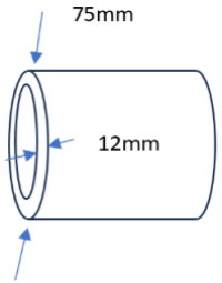
Figure 1. Sketch of mild steel pipe used for Butt joint welding.
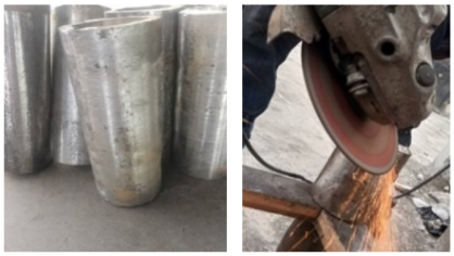
Figure 2. Sample preparation.
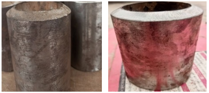
Figure 3. Finished coupon.
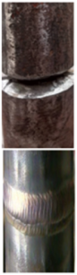
Figure 4. Welded joint.
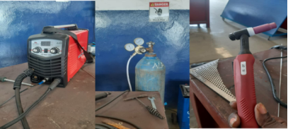
Figure 5. TIG/MMA-250S Welding Machine and other Equipment.
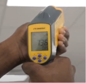
Figure 6. Fluke62 Max infrared thermometer.
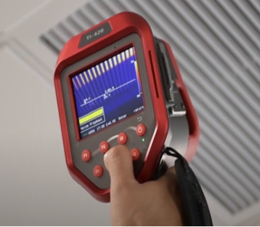
Figure 7. FLIR System-GF304 thermography.
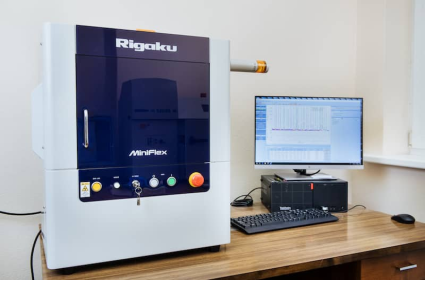
Figure 8. AutoMATE II X-ray diffraction device.
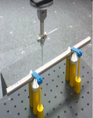
Figure 9. Coordinate Measuring machine (CMM).
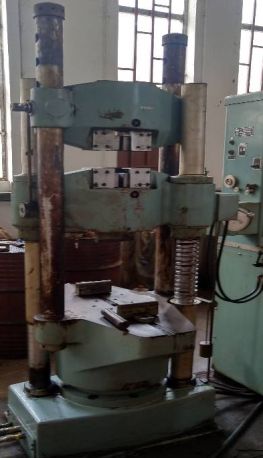
Figure 10. M0565SHIMADZU UNIVERSAL TESTING MACHINE (UTM).
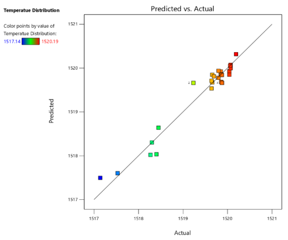
Figure 11. Peak Temperature.
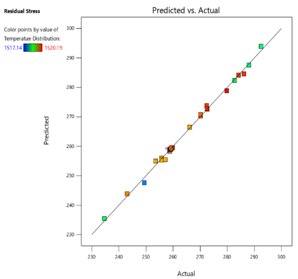
Figure 12. Residual stress.
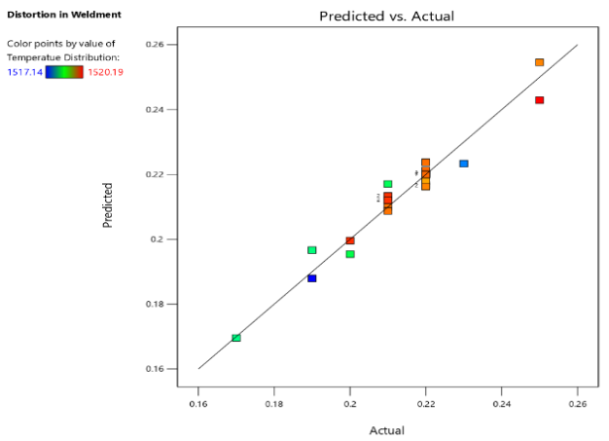
Figure 13. Distortion in weldment.
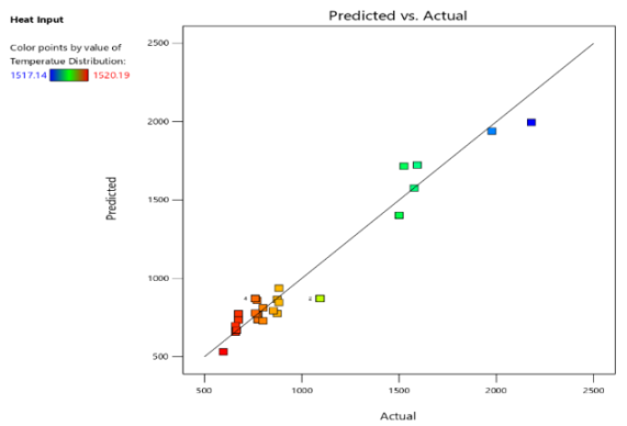
Figure 14. Heat flux.
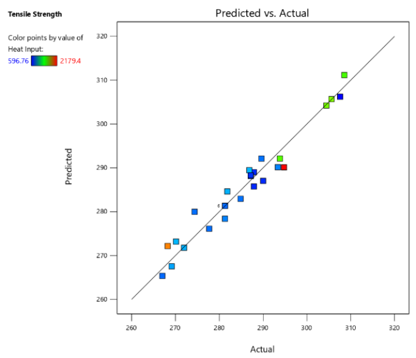
Figure 15. Tensile strength.
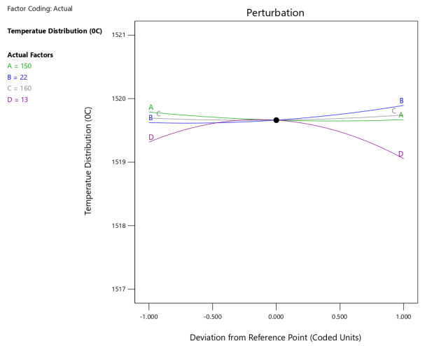
Figure 16. Perturbation plot for Peak Temperature.
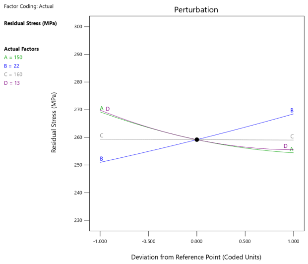
Figure 17. Perturbation plot for residual stress.

Figure 18. Perturbation plot for distortion in weldment.
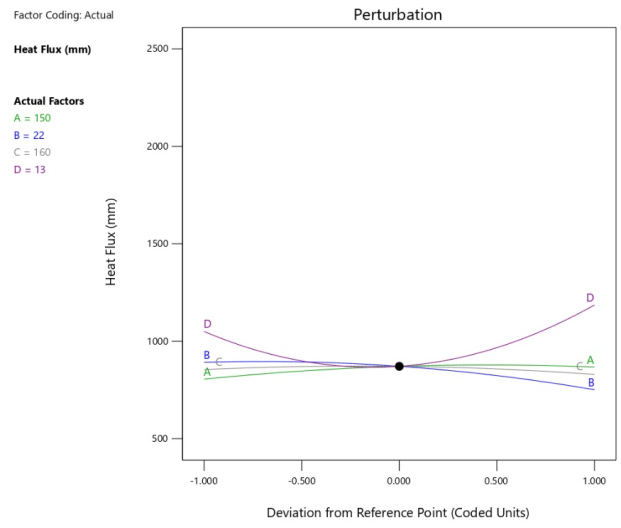
Figure 19. Perturbation plot for heat flux.
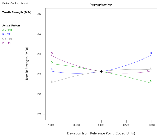
Figure 20. Perturbation plot for tensile strength.
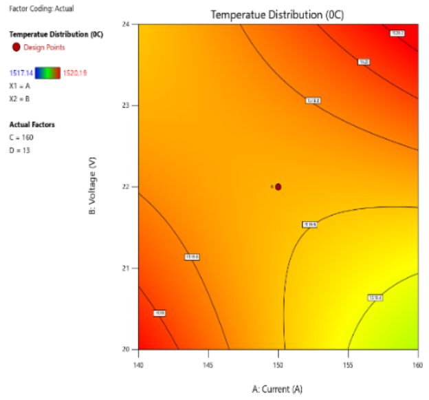
Figure 21. Contour plot for Peak Temperature.
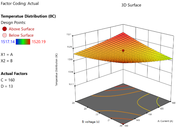
Figure 22. 3D surface plot for Peak Temperature.
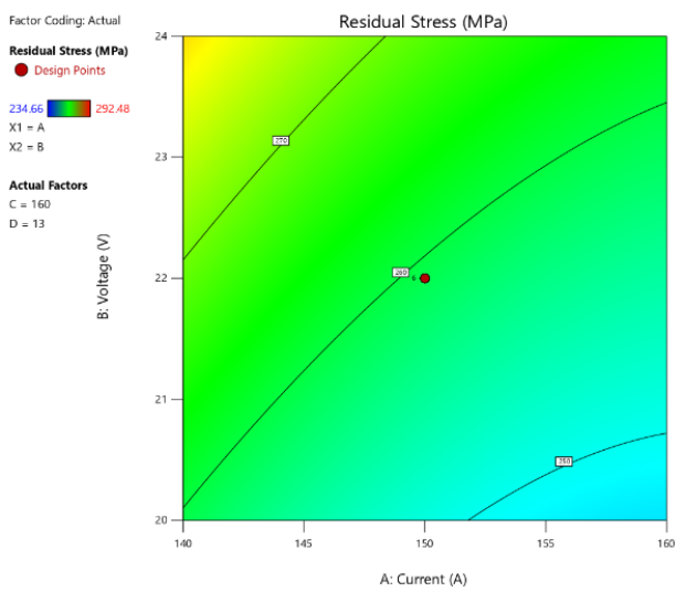
Figure 23. Contour plot for Residual Stress.

Figure 24. 3D surface plot for Residual Stress.

Figure 25. Contour plot for Distortion in Weldment.
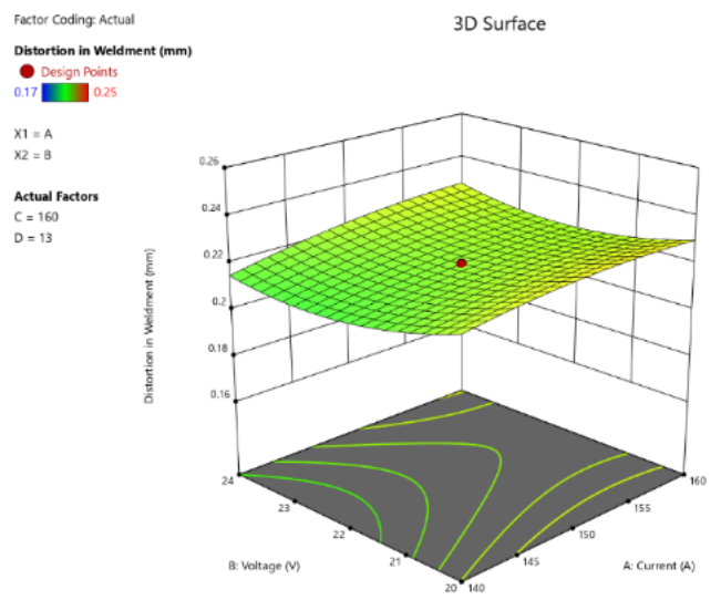
Figure 26. 3D plot for Distortion in Weldment.
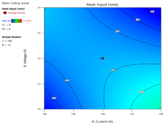
Figure 27. Contour plot for Heat Flux.
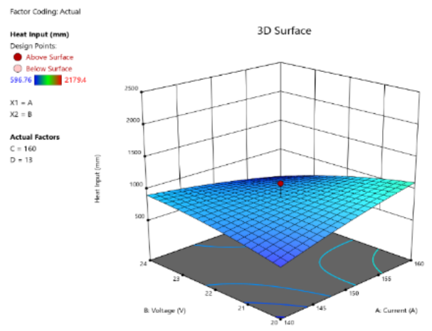
Figure 28. 3D surface plot for Heat Flux.
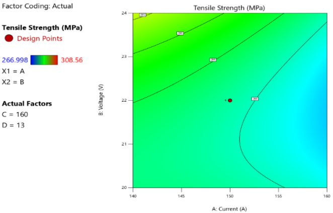
Figure 29. Contour plot for Tensile strength.
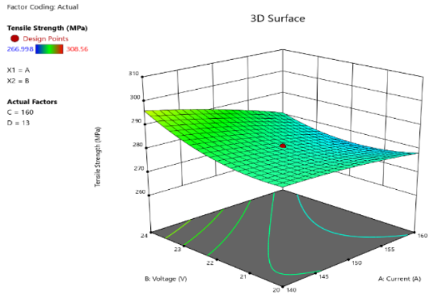
Figure 30. 3D surface plot for Tensile strength.
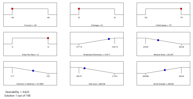
Figure 31. RSM Ramps Optimization diagram.
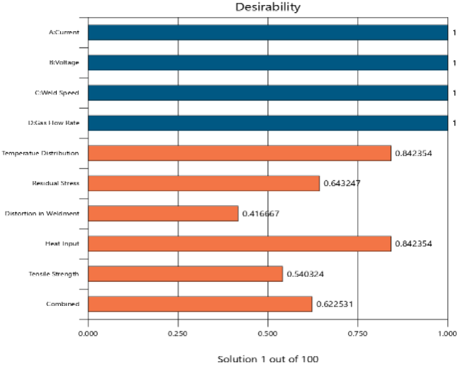
Figure 32. RSM Bar graph for Optimization.
Information