Phenomena of Inertia Bias in Research, Practicalities of Possible Adjustment

Oleksandr Ocheredko

doi:doi:10.11648/j.ajhr.20241206.14

Research Article |

| Peer-Reviewed

Phenomena of Inertia Bias in Research, Practicalities of Possible Adjustment

Oleksandr Ocheredko^*

Published in American Journal of Health Research (Volume 12, Issue 6)

Received: 1 October 2024 Accepted: 12 November 2024 Published: 21 November 2024

Views: Downloads:

Download PDF

Share This Article

Twitter
Linked In
Facebook

Abstract

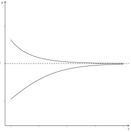
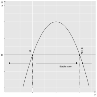
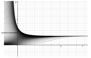
In academic research, bias refers to a type of systematic error that can distort measurements and/or affect investigations and their results. Biases can be present in both quantitative and qualitative research. The common effect of biases is undermining the power of statistical tests, therefore findings induced to support H0 hypothesis. Corrections depend on nature of bias and aimed to recover magnitude of association. Corrections use analytical constructs therefore applied in data analysis stage. Considered in the paper is of novel type and tentatively named inertia bias. This bias is of directed uncertainty about true value of index. One can find it in the range of designs and measures. The essence is the exposure takes time to shift index to new equilibrium. The problem is that researcher usually unaware of time required for index to settle down at new equilibrium. Therefore one inevitably measures the transition states instead of equilibrium yielding different magnitudes of attenuated association. How to obtain measure equilibrium value is the focus of the paper. Given the dynamical setup I referred to first order nonlinear differential equations, in particular logistic differential equation that meats necessary prerequisites: it should be separable equation, it has to have stable state, solutions have to descend or ascend toward equilibrium with the tangency in time. This paper describes range of circumstances where researcher faces the problem along with suggested solution, calculus, and tested software.

Published in	American Journal of Health Research (Volume 12, Issue 6)
DOI	10.11648/j.ajhr.20241206.14
Page(s)	186-192
Creative Commons	This is an Open Access article, distributed under the terms of the Creative Commons Attribution 4.0 International License (http://creativecommons.org/licenses/by/4.0/), which permits unrestricted use, distribution and reproduction in any medium or format, provided the original work is properly cited.
Copyright	Copyright © The Author(s), 2024. Published by Science Publishing Group

Keywords

Bias, Equilibrium, Stable State, Logistic Differential Equation

1. Introduction

Biases are pervasive and different in nature

[1, 2]

. Usually they come together in a study shifting results unpredictably [3, 4]. No design of data collection is free of at least some particular biases pertaining to it

[5-7]

. This requires corrections that complicate both data analysis and deductions

[8, 9].

This paper describes new type of bias, suggestive name is inertia bias. Along with selection and measurement biases It’s pervasive and occurs in different designs and settings.

2. Materials and Methods

2.1. Major Known Biases

Biases spread around different fields of disciplines and researches

[10, 11]

. Typical but somewhat arbitrary and incomplete classification of biases is:

Information bias (Recall bias, Observer bias, Performance bias, Regression to the mean)

Interviewer bias

Publication bias

Researcher bias

Response bias (Acquiescence bias, Demand bias, Social desirability bias, Courtesy bias, Question order bias, Extreme responding bias)

Selection bias (Sampling or ascertainment bias, Berkson’s bias, Attrition bias, Self-selection or volunteer bias, nonresponse bias, Survivorship bias, Undercoverage bias, competing risk bias)

Cognitive bias (Anchoring bias, Primacy bias, Framing effect, Actor–observer bias, Availability heuristic, Confirmation bias, halo effect)

Hawthorne effect

Observer bias

Omitted Variable Bias

Pygmalion effect

Placebo Effect

Censoring & truncation bias

Measurement bias

Construct bias

Some of these biases corrections based on analytical tools, whereas others are preferably attenuated by data collection refinements.

2.2. The Nature of Inertia Bias

Let’s consider Clinical Trial with placebo and active treatment groups. You take information on some index at the start and some period t1 after for both groups and make comparison. Say, difference is

△_{t 1}

. Would it be the same if You made measurements at period t2? What about

△_{t 3}

Response development is not immediate but rather dynamic and so we have possible situations graphed in Figure 1.

Example 1. The Lifestyle Heart Trial (1990)

[12]

In the Lifestyle Heart Trial subjects with angiographically documented coronary heart disease were randomly assigned to an experimental or a usual-care group. Experimental subjects were prescribed a low-fat vegetarian diet, moderate aerobic exercise, stress management training, stopping smoking and group support. The usual-care subjects were not asked to change their lifestyle. Progression or regression of coronary artery lesions was assessed in both groups by angiography at baseline, after a year, and after 5 years. In the experimental group, the average percent stenosis decreased from 40.7% at baseline to 38.5% at 1 year to 37.3% at 5 years (a 7.9% relative improvement). In the control group, the percent stenosis increased from 41.3% to 42.3% at 1 year to 51.9% at 5 years (a 27.7% relative worsening) (between-group differences, p=0.001 at 5 years). More regression of coronary atherosclerosis occurred after 5 years in the experimental group, while in the control group, coronary atherosclerosis progression continued and more than twice as many cardiac events occurred.

There are two uncertainties what is the final effect and whether we have stable environment in 1 and along 5 years. That bring a question of inertia bias.

Download: Download full-size image

Figure 1. Dynamics of index to equilibrium,

\bar{y}

To measure index correctly we have to evaluate it on equilibrium. The problem is that we don’t know the time when equilibrium is reached. Theoretically it’s infinite time to be sure but in practice we can’t wait too long because other influential events can happen.

It stands to reason that panel data too don’t guarantee reaching equilibrium for it can be temporal state.

Example 2. Danish women management performance panel study (2006)

[13]

The study examines the relationship between management diversity and firm performance for the 2500 largest Danish firms observed during the period 1992– 2001. «We estimate various panel data models of firm performance and control for factors that are traditionally found to affect firm performance e.g. firms’ age, size, sector, export orientation.» Researched found that «the proportion of women among top executives and on boards of directors tends to have a significantly positive effect on firm performance». However, when controlling for unobserved firm-specific factors, «the effect often turns insignificant … due to large statistical uncertainty».

I suggest the presence of inertia bias for potential influence of previous management policies and inertia of outcome measures due to complexity of the processes. Elicitation of true influence can help break through «large statistical uncertainty» if indeed the true effect is of magnitude.

To the greater extend inertia bias problem applied to less informative «snapshot» designs, for example correlational (ecological) studies.

2.3. Correction for Inertia Bias

2.3.1. Equilibrium

Equilibrium is theoretical notion for there is no practical tools to measure it directly. Therefore the only recourse I can think of is analytical correction.

I opted for simplest differential equation that suggests one steady state (that is equilibrium) and describes range of processes similar in building up to current problem. This is logistic differential equation:

\frac{\partial y}{\partial t} = αy (t) - βy (t)^{2}

α, β > 0

(1)

The two possible solutions at

\frac{\partial y}{\partial t}

= 0 are

y(t)=0andy(t)=

\frac{α}{β}

,(2)

These are demonstrated by Figure 2

Download: Download full-size image

Figure 2. Two equilibrium solutions.

Figure 2 shows that all non-constant solutions approach the equilibrium solution y(t) =

\frac{α}{β}

t \to \infty

, some from above the line

\bar{y} = \frac{α}{β}

and others from below (see Figure 3). Another solution 0 is not steady state and has nothing to do with equilibrium.

Solutions to logistic differential equation with parameters

α

and

β

are graphed on Figure 3.

Solutions presented by Figure 3 described by formula

y (t) = \frac{y_{0} α e^{αt}}{α - y_{0} β + y_{0} β e^{αt}}

(3)

Where parameters

α

and

β

define solution curves while initial condition

y_{0}

defines particular curve. The index value at the beginning of treatment corresponds to zero time (t=0) that defines relationship between

α

and

β

. To solve You need just another trajectory point, say index measured in month.

2.3.2. Examples

I delivered possible ways of arriving at solutions with 2 simulated examples. Simulation is used to check for correctness of solutions of course.

Example 1

Let’s check for known equation

y' = 2 y - y^{2}

y_{0}

= 1, so that

α

= 2 and

β

= 1,

y_{0}

< 2.

Trajectory of index then described as:

y (t) = \frac{2 e^{2 t}}{1 + e^{2 t}}

(4)

Download: Download full-size image

Figure 3. Solutions to logistic differential equation.

Let’s generate y for t = 0, 1, …, 10. We have y= 1.0, 1.761594, 1.964028, 1.995055, 1.999329, 1.999909, 1.999988, 1.999998, 2.0, 2.0, 2.0

Suppose we observed just 2 values at times 1 and 2, so they are 1.761594, 1.964028

Given information on times (t=1, 2) and values of index (y= 1.761594, 1.964028) let’s find equilibrium which we know by setup is 2/1=2

Example 2

Let’s check for known equation

y' = 2 y - y^{2}

y_{0}

= 3, so that again

α

= 2 and

β

= 1., but

y_{0}

> 2

Trajectory of index then described as:

y (t) = \frac{6 e^{2 t}}{1 + 3 e^{2 t}}

(5)

Let’s generate y for t = 0, 1, …, 10. We have y= 3.0, 2.094486, 2.012285, 2.001654, 2.000224, 2.000030, 2.000004, 2.000001, 2.0, 2.0, 2.0.

Suppose we observed 2 values at times 1 and 3, so they are 2.094486, 2.001654.

Given information on times (t=1, 3) and values of index (y= 2.094486, 2.001654) let’s again find equilibrium 2.

2.3.3. Solutions and R Software

For the solutions I used exclusively R

[14]

based software, whereas one can find more elaborate routines with Mathematica, MATLAB, Mathcad, Python, Excel based software.

First of all, calculus by hand and linearisation with subsequent solution with functions solve(), backsolve(), qr.solve() of «base» package, or similars are proved to be dead ends.

So I used solvers of systems of non-linear equations, i.e., function nleqslv() of package «nleqslv» [15, 16], function multiroot() of package «rootSolve» [17]. Another alternative is to use optimisation routines rendered by R based functions optim() and nlm() of package «stats» [18]. You can use solvers of systems of non-linear equations with and without Jacobian. Jacobian for (3) is of two derivatives:

\frac{\partial y}{\partial α} = 1 - \frac{y_{0} αt e^{αt}}{y (t)} - \frac{y_{0} e^{αt}}{y (t)} + y_{0} βt e^{αt}

\frac{\partial y}{\partial β} = y_{0} (e^{αt} - 1)

(6)

Code of data (y1, y2) generation given Examples1&2:

Indexes1<-function(t){

l<-length(t)

y<-numeric(l)

y<-2*exp(2*t)/(1+exp(2*t))

}

indexes2<-function(t){

l<-length(t)

y<-numeric(l)

y<-6*exp(2*t)/(-1+3*exp(2*t))

}

t<-array(0:10)

y1<-indexes1(t)

y2<-indexes2(t)

(i). Solution with Nleqslv

Solution code using nleqslv(), example 1:

library(nleqslv)

xstart <- c(10,10)

C=1 #y0

Y=c(1.76159, 1.964028) #observed Y at times =1, 2

t=c(1,2)

dslnex1 <- function(x) {

e <- numeric(2)

e[1] <- x[1] - C*x[2] +C*x[2]*exp(t[1]*x[1]) - (C/Y[1])*x[1]*exp(t[1]*x[1])

e[2] <- x[1] - C*x[2] +C*x[2]*exp(t[2]*x[1]) - (C/Y[2])*x[1]*exp(t[2]*x[1])

}

# Jacobian definition

Jac <- function(x) {

J <- matrix(0,nrow=2,ncol=2)

J[,1] <- c(1+C*x[1]*t[1]*exp(t[1]*x[2]) - C*t[1]*x[2]*exp(t[1]*x[2])/Y[1] - C*exp(t[1]*x[2])/Y[1], C*exp(t[1]*x[2])-C)

J[,2] <- c(1+C*x[1]*t[2]*exp(t[2]*x[2]) - C*t[2]*x[2]*exp(t[2]*x[2])/Y[2] - C*exp(t[2]*x[2])/Y[2], C*exp(t[2]*x[2])-C)

}

nles<-nleqslv(xstart, dslnex1, control=list(trace=1,btol=.01,delta="cauchy"))

# OR with Jacobian to the same result

nlesJ<-nleqslv(xstart, dslnex1, Jac, method="Broyden", global="none", control=list(trace=1,stepmax=2))

(ii). Solution with Rootsolve

Solution code using rootSolve(), example 1:

library(rootSolve)

model <- function(x) {

F1 <- x[1] - 1*x[2] +1*x[2]*exp(1*x[1]) - (1/1.76159)*x[1]*exp(1*x[1])

F2 <- x[1] - 1*x[2] +1*x[2]*exp(2*x[1]) - (1/1.964)*x[1]*exp(2*x[1])

c(F1 = F1, F2 = F2)

}

roots <- multiroot(f = model, start = xstart)

# OR with Jacobian to the same result

rootsJ<- multiroot(f = model, start = xstart, jacfunc = Jac)

(iii). Solutions with Optimisers

Solution code using optim(), nlm() example 1:

fn <- function(a, b) {

eq1 <- C*a*exp(a*t[1])/(a-C*b+C*b*exp(a*t[1]))

eq2 <- C*a*exp(a*t[2])/(a-C*b+C*b*exp(a*t[2]))

return(c(eq1, eq2) )

}

fn2 <- function(x) crossprod( fn(x[1], x[2]) - Y)

ops<-optim(xstart, fn2)

nlm<-nlm(f=fn2, p=xstart)

solutions<-list(start=xstart, rootSolve= roots$root, rootSolve_J=r rootsJ$root,

nleqslv= nles$x, optim=ops$par, nlm=nlm$estimate)

The last line of code pulls together solutions from different solvers to be compared together with initial values of parameters

α

and

β

3. Results

Results for initial values of

α

=10 and

β

=10 from different solvers are presented in Table 1. Choosing these initial parameters values is the case of «blank» information as to comparative magnitude plus scaling up by order 1.

Table 1. Equilibrium estimations by different solvers with initial parameters values of

α

=10 and

β

=10.

Initial 10,10	Example 1 (4)			Example 2 (5)
Solvers	alpha	beta	Equilibrium	alpha	beta	Equilibrium
rootSolve	2.000096	1.000066	1.999964	2.000096	1.000066	1.999964
rootSolve_J	2.000096	1.000066	1.999964	2.000096	1.000066	1.999964
nleqslv	1.9999722	0.9999848	2.000003	2.000001	1	2
optim	12.950431	6.952232	1.862773	13.455259	6.569881	2.048022
nlm	1.9999832	0.9999912	2.000001	13.189039	6.439741	2.04807

I also checked for influence of discrepancy in initial

α

and

β

ratio with true value of 2, given as 5 by initial parameters values of

α

=10 and

β

=2. This is quite possible in practicalities. Results are given in Table 2.

Table 2. Equilibrium estimations by different solvers with initial parameters values of

α

=10 and

β

=2.

Initial 10,2	Example 1 (4)			Example 2 (5)
Solvers	alpha	beta	Equilibrium	alpha	beta	Equilibrium
rootSolve	2.000096	1.000066	1.999964	2.000096	1.000066	1.999964
rootSolve_J	2.000096	1.000066	1.999964	2.000096	1.000066	1.999964
nleqslv	1.9999722	0.9999848	2.000003	2.000001	1	2
optim	2.001468	1.000773	1.999922	2.002238	1.001078	2.000082
nlm	48.97191	26.28929	1.862809	48.75963	23.80760	2.04807

Finally, I tried the worst scenario given the reverse ratio of 0.5 by initial parameters values of

α

=1 and

β

=2. This is rare possibility but still worthwhile to consider given controversial hypothesis testing. Results are displayed in Table 3.

Table 3. Equilibrium estimations by different solvers with initial parameters values of

α

=1 and

β

=2.

Initial 1,2	Example 1 (4)			Example 2 (5)
Solvers	alpha	beta	Equilibrium	alpha	beta	Equilibrium
rootSolve	2.000096	1.000066	1.999964	2.000096	1.000066	1.999964
rootSolve_J	2.000096	1.000066	1.999964	2.000096	1.000066	1.999964
nleqslv	1.9999722	0.9999848	2.000003	0	3.9226e-21	0
optim	2.001468	1.000773	1.999922	1.9990474	0.9995273	1.999993
nlm	48.97191	26.28929	1.862809	2.000006	1.000003	2

4. Discussion

Pervasive nature of inertia bias requires attention and remedial action. Suggested approach is based on processing dynamics of indexes toward reaching equilibrium. From simulated examples it seems that differential equation solutions meet the purpose. I have used simplest logistic equation just to demonstrate idea. It has 2 solutions, one is zero describes unstable state, while another stable state, or equilibrium, see Figures 2 and 3. Stable state is what we seek. Figure 1 graphs two possible situations that engender two examples. One related to growing index value, another pertains to falling magnitude. Consider Example 1 of 2.2. In the experimental group, the average percent stenosis decreased from 40.7% at baseline to 38.5% at 1 year to 37.3% at 5 years (a 7.9% relative improvement). In the control group, the percent stenosis increased from 41.3% to 42.3% at 1 year to 51.9% at 5 years (a 27.7% relative worsening). Experimental group index was decreasing whereas in controls it was increasing. Simulated examples of 2.3.2. follow the suit. First example has initial value

y_{0}

=1 less then equilibrium value 2, whereas second has initial value

y_{0}

=3 above equilibrium.

I purposely illustrated performance of different solvers under different initial parameters

α

and

β

. Table 1 data examine performance given equal initial parameters values, i.e., the case of information insufficiency. I would conclude similarity and good performance across solvers. Information on Jacobian seems to be dispensable for routines.

Situation with huge bias in hypothesised equilibrium value is illustrated by applying initial

α

and

β

values of 10 and 2 with ratio 5 that is far from 2. Results from 2 models are combined in Table 2. Still good performance across solvers. One may notice that some solvers yield incorrect estimates of

α

and

β

parameters. As long as equilibrium estimates are good why bother.

α

and

β

values per se are of no considerations.

Finally, I put through scenario given the reverse ratio of 0.5 by initial parameters values of

α

=1 and

β

=2. Table 3 data signalise the only trouble with nleqslv solver that stalemated with zero solution in descending dynamics.

I emphasise once more on didactic purpose of paper without trying to dig in depth of more complex or general differential equations. You can do better. I also presented performance of narrow set of common solvers. I obtained same results with some other solvers. For that matter I used NLSOLVE() Excel function, and even on-line solvers but opted not to clutter the text.

5. Conclusions

Inertia bias is novel type and first time introduced in the paper. It is ubiquitous in both ecological and longitudinal studies and should be taken care of. It is caused by incidental measurements of indexes in transition toward equilibrium of which we are unaware on most part.

Incidental measurements while being compared bring incidental effects, instead one should compare equilibrium values.

Suggested solution relates to obtaining stable states of differential equations describing index dynamic. In paper logistic equation considered.

Common solvers evince good performance with a wide set of initial values of parameters.

Author Contributions

Oleksandr Ocheredko is the sole author. The author read and approved the final manuscript.

Conflicts of Interest

The author declares no conflicts of interest.

References

[1]	Popovic A., Huecker, M. Study Bias. In: StatPearls [Internet]. Treasure Island (FL): StatPearls Publishing; 2024. PMID: 34662027 Bookshelf ID: NBK574513.
[2]	Florczak, K. Best Available Evidence or Truth for the Moment: Bias in Research. //Nursing Science Quarterly. Volume 35 Issue 1, 2022, pp. 20–24. https://doi.org/10.1177/0894318421105
[3]	Arias, F., Navarro, M., Elfanagely, Y. Elfanagely, O. Biases in research studies. In: Handbook for Designing and Conducting Clinical and Translational Research, 2023, Ch. 31, pp. 191-194.
[4]	Odonnat, A., Feofanov, V., Redko, I. Leveraging Ensemble Diversity for Robust Self-Training in the Presence of Sample Selection Bias./ 27th International Conference on Artificial Intelligence and Statistics, AISTATS 2024; Valencia; Spain; 2-4 May 2024. In: Proceedings of Machine Learning Research. Vol. 238, 2024, pp. 595-603.
[5]	Jabarov, J. Bias in scientific research: How to identify and eliminate it. Journal of Science and Innovative Technologies International Scientific Research Journal. Issue 25, 2023, pp. 80-96. https://doi.org/10.30546/2616-4418.25.2023.80
[6]	Zheng, B. Ordinary Differential Equation and Its Application. In: Highlights in Science, Engineering and Technology. Vol. 72, 2023, pp. 645-65. https://doi.org/10.54097/rnnev212
[7]	Henner, V., Nepomnyashchy, A., Belozerova, T. Ordinary Differential Equations: Analytical Methods and Applications. Springer, 2023, p.608.
[8]	Magnus, R. Essential Ordinary Differential Equations. Springer, 2023, p.283.
[9]	Simundi, A-M. Bias in research. Biochemia Medica. 2013 23(1): 12-15. https://doi.org/10.11613/BM.2013.003
[10]	Smith, J., Noble, H. (2014). Bias in research. Evidence-Based Nursing, 17(4), 100-101. https://doi.org/10.1136/eb-2014-101946
[11]	Hunter, J., Schmidt, F. Methods of Meta-Analysis Corrected Error and Bias in Research Findings. Journal of the American Statistical Association. Vol. 86, No. 413(Mar., 1991), pp. 242-244 https://doi.org/10.2307/2289738
[12]	Ornish, D., Scherwitz, L.W., Billings, J.H., Brown S.E., Gould, K. L., Merritt, T.A., Sparler, S., Armstrong, W. T., Ports, T. A., Kirkeeide, R.L., Hogeboom, C., Brand, R.J. Intensive lifestyle changes for reversal of coronary heart disease. JAMA. 1998 Dec 16; 280(23): 2001-7. https://doi.org/10.1001/jama.280.23.2001
[13]	Smith, N., Smith, V. and Verner, M. (2006), "Do women in top management affect firm performance?A panel study of 2,500 Danish firms", International Journal of Productivity and Performance Management, Vol. 55 No. 7, pp. 569-593. https://doi.org/10.1108/17410400610702160
[14]	The R Project for Statistical Computing. https://www.r-project.org/
[15]	Aitkin, M., Francis, B., Hinde,J., Darnell, R. (2023). Statistical Modelling in R. Oxford University Press, 553. https://doi.org/10.1093/oso/9780199219148.001.0001
[16]	Hasselman,B. (2003) Package ‘nleqslv’. https://cran.r-project.org/web/packages/nleqslv/nleqslv.pdf
[17]	Karline Soetaert, K., Hindmarsh, A., Eisenstat, S. C., et.al. (2003). Package ‘rootSolve’. https://cran.r-project.org/web/packages/rootSolve/rootSolve.pdf
[18]	R Core Team. (2024). Package «stats». https://stat.ethz.ch/R-manual/R-devel/library/stats/html/00Index.html

Cite This Article

Plain Text BibTeX RIS

APA Style

Ocheredko, O. (2024). Phenomena of Inertia Bias in Research, Practicalities of Possible Adjustment. American Journal of Health Research, 12(6), 186-192. https://doi.org/10.11648/j.ajhr.20241206.14

Copy | Download

ACS Style

Ocheredko, O. Phenomena of Inertia Bias in Research, Practicalities of Possible Adjustment. Am. J. Health Res. 2024, 12(6), 186-192. doi: 10.11648/j.ajhr.20241206.14

Copy | Download

AMA Style

Ocheredko O. Phenomena of Inertia Bias in Research, Practicalities of Possible Adjustment. Am J Health Res. 2024;12(6):186-192. doi: 10.11648/j.ajhr.20241206.14

Copy | Download

@article{10.11648/j.ajhr.20241206.14,
  author = {Oleksandr Ocheredko},
  title = {Phenomena of Inertia Bias in Research, Practicalities of Possible Adjustment
},
  journal = {American Journal of Health Research},
  volume = {12},
  number = {6},
  pages = {186-192},
  doi = {10.11648/j.ajhr.20241206.14},
  url = {https://doi.org/10.11648/j.ajhr.20241206.14},
  eprint = {https://article.sciencepublishinggroup.com/pdf/10.11648.j.ajhr.20241206.14},
  abstract = {In academic research, bias refers to a type of systematic error that can distort measurements and/or affect investigations and their results. Biases can be present in both quantitative and qualitative research. The common effect of biases is undermining the power of statistical tests, therefore findings induced to support H0 hypothesis. Corrections depend on nature of bias and aimed to recover magnitude of association. Corrections use analytical constructs therefore applied in data analysis stage. Considered in the paper is of novel type and tentatively named inertia bias. This bias is of directed uncertainty about true value of index. One can find it in the range of designs and measures. The essence is the exposure takes time to shift index to new equilibrium. The problem is that researcher usually unaware of time required for index to settle down at new equilibrium. Therefore one inevitably measures the transition states instead of equilibrium yielding different magnitudes of attenuated association. How to obtain measure equilibrium value is the focus of the paper. Given the dynamical setup I referred to first order nonlinear differential equations, in particular logistic differential equation that meats necessary prerequisites: it should be separable equation, it has to have stable state, solutions have to descend or ascend toward equilibrium with the tangency in time. This paper describes range of circumstances where researcher faces the problem along with suggested solution, calculus, and tested software.
},
 year = {2024}
}

Copy | Download

TY - JOUR
T1 - Phenomena of Inertia Bias in Research, Practicalities of Possible Adjustment

AU - Oleksandr Ocheredko
Y1 - 2024/11/21
PY - 2024
N1 - https://doi.org/10.11648/j.ajhr.20241206.14
DO - 10.11648/j.ajhr.20241206.14
T2 - American Journal of Health Research
JF - American Journal of Health Research
JO - American Journal of Health Research
SP - 186
EP - 192
PB - Science Publishing Group
SN - 2330-8796
UR - https://doi.org/10.11648/j.ajhr.20241206.14
AB - In academic research, bias refers to a type of systematic error that can distort measurements and/or affect investigations and their results. Biases can be present in both quantitative and qualitative research. The common effect of biases is undermining the power of statistical tests, therefore findings induced to support H0 hypothesis. Corrections depend on nature of bias and aimed to recover magnitude of association. Corrections use analytical constructs therefore applied in data analysis stage. Considered in the paper is of novel type and tentatively named inertia bias. This bias is of directed uncertainty about true value of index. One can find it in the range of designs and measures. The essence is the exposure takes time to shift index to new equilibrium. The problem is that researcher usually unaware of time required for index to settle down at new equilibrium. Therefore one inevitably measures the transition states instead of equilibrium yielding different magnitudes of attenuated association. How to obtain measure equilibrium value is the focus of the paper. Given the dynamical setup I referred to first order nonlinear differential equations, in particular logistic differential equation that meats necessary prerequisites: it should be separable equation, it has to have stable state, solutions have to descend or ascend toward equilibrium with the tangency in time. This paper describes range of circumstances where researcher faces the problem along with suggested solution, calculus, and tested software.

VL - 12
IS - 6
ER -

Copy | Download

Author Information

Oleksandr Ocheredko

Social Medicine and Health Services Administration Department, Vinnytsia National Pirogov Medical University, Vinnytsia, Ukraine

Biography: Oleksandr Ocheredko is a chair of Social Medicine and Health Services Administration Department at National Pirogov Memorial Medical University, Vinnytsya, Ukraine. He completed his PhD in Social Medicine and Health Services Administration from Bogomolets National Medical University in 1995, and obtained full Doctorate of Medical Science in 2004. Was invited lecturer in Public Health School at Iowa State University in 2005. Since 2007 he is honoured with national professor degree. He is ISDSA member, maintainer of R package «ltable», currently serves on the Editorial Boards of Journal of Behavioral Data Science, US, as well as 4 Editorial Boards of national journals.

Research Fields: (1) Optimisation approach in Social Medicine and Health Services, (2) Data Science and Analytics in particular Power Analysis, Equilibrium Exploration, (3) Health Economics & Econometrics in particular applied economic analyses in Health Research, (4) Evidence based Clinical Medicine and Evidence based Public Health in particular meta-analysis, (5) MCMC algorithms, in particular stationarity detection.

Contact Email

http://orcid.org/0000-0002-4792-8581

Download PDF

Plain Text BibTeX RIS

APA Style

Ocheredko, O. (2024). Phenomena of Inertia Bias in Research, Practicalities of Possible Adjustment. American Journal of Health Research, 12(6), 186-192. https://doi.org/10.11648/j.ajhr.20241206.14

Copy | Download

ACS Style

Ocheredko, O. Phenomena of Inertia Bias in Research, Practicalities of Possible Adjustment. Am. J. Health Res. 2024, 12(6), 186-192. doi: 10.11648/j.ajhr.20241206.14

Copy | Download

AMA Style

Ocheredko O. Phenomena of Inertia Bias in Research, Practicalities of Possible Adjustment. Am J Health Res. 2024;12(6):186-192. doi: 10.11648/j.ajhr.20241206.14

Copy | Download

@article{10.11648/j.ajhr.20241206.14,
  author = {Oleksandr Ocheredko},
  title = {Phenomena of Inertia Bias in Research, Practicalities of Possible Adjustment
},
  journal = {American Journal of Health Research},
  volume = {12},
  number = {6},
  pages = {186-192},
  doi = {10.11648/j.ajhr.20241206.14},
  url = {https://doi.org/10.11648/j.ajhr.20241206.14},
  eprint = {https://article.sciencepublishinggroup.com/pdf/10.11648.j.ajhr.20241206.14},
  abstract = {In academic research, bias refers to a type of systematic error that can distort measurements and/or affect investigations and their results. Biases can be present in both quantitative and qualitative research. The common effect of biases is undermining the power of statistical tests, therefore findings induced to support H0 hypothesis. Corrections depend on nature of bias and aimed to recover magnitude of association. Corrections use analytical constructs therefore applied in data analysis stage. Considered in the paper is of novel type and tentatively named inertia bias. This bias is of directed uncertainty about true value of index. One can find it in the range of designs and measures. The essence is the exposure takes time to shift index to new equilibrium. The problem is that researcher usually unaware of time required for index to settle down at new equilibrium. Therefore one inevitably measures the transition states instead of equilibrium yielding different magnitudes of attenuated association. How to obtain measure equilibrium value is the focus of the paper. Given the dynamical setup I referred to first order nonlinear differential equations, in particular logistic differential equation that meats necessary prerequisites: it should be separable equation, it has to have stable state, solutions have to descend or ascend toward equilibrium with the tangency in time. This paper describes range of circumstances where researcher faces the problem along with suggested solution, calculus, and tested software.
},
 year = {2024}
}

Copy | Download

TY - JOUR
T1 - Phenomena of Inertia Bias in Research, Practicalities of Possible Adjustment

VL - 12
IS - 6
ER -

Copy | Download