Representation with Index Matrices Discrete Random Variables

Stela Todorova

doi:doi:10.11648/j.ajam.20251301.14

Research Article |

| Peer-Reviewed

Representation with Index Matrices Discrete Random Variables

Stela Todorova^*

Published in American Journal of Applied Mathematics (Volume 13, Issue 1)

Received: 4 January 2025 Accepted: 18 January 2025 Published: 10 February 2025

Views: Downloads:

Download PDF

Share This Article

Twitter
Linked In
Facebook

Abstract

With the Theory of probabilities it is made a mathematical description of a finite set of probability trials with random outcomes. Basically, the results from a given laboratory experiment are illustrated with tables, diagrams, ordinary matrices. Index matrices are a new approach of presenting and analyzing information of data. In this article the author will represent with Index Matrices, which elements are real numbers; function-type of elements, with which results of formulas with different parameters can be calculated and predicates, with which can be checked if a random outcome meets certain conditions according to a finite set of interval order. In order the data that we analyze to be more precisely verified, is not only ordered sequentially, but also a result of calculation of parameters from a given diapason at equal intervals. In this way the number of desired outcomes can be compared with not desired outcomes and with the data from different experiments, which can result in prediction of alternative values in the future. An illustration with Excel is described with an Index matrix, which elements are voltages between 0 and a value read by analog pin of Arduino Uno board, which is also presented with X and Y axis of a Chart diagram.

Published in	American Journal of Applied Mathematics (Volume 13, Issue 1)
DOI	10.11648/j.ajam.20251301.14
Page(s)	57-63
Creative Commons	This is an Open Access article, distributed under the terms of the Creative Commons Attribution 4.0 International License (http://creativecommons.org/licenses/by/4.0/), which permits unrestricted use, distribution and reproduction in any medium or format, provided the original work is properly cited.
Copyright	Copyright © The Author(s), 2025. Published by Science Publishing Group

Keywords

Index Matrix, Theory of Probability, Random Variables, Algebra of Events, Probability of Trials, Arduino

1. Introduction

Let

I

be a fixed set of indices and  be the set of the real numbers. Let the standard sets

K

and

L

satisfy the condition:

K, L \subset I

. Let over these sets, the standard set-theoretical operations be defined. We call “IM with real number elements” (R-IM) the object:

where

K = \{k_{1}, k_{2}, . . ., k_{m}\}

and

L = \{l_{1}, l_{2}, . . ., l_{n}\}

, and for

1 \leq i \leq m

, and

1 \leq j \leq n : a_{k_{i}, l_{j}} \in R

When set

R

is changed with set {0, 1}, we obtain a particular case of an IM with elements being real numbers, that we denote by (0, 1)-IM.

When we choose to work with matrices, elements of which are logical variables, propositions or predicates – let us call these IM “Logical IMs (L-IMs)”.

Let the set of all used functions be Ƒ. The research over of this document.

IMs with function-type of elements has two cases:

1. each function of set Ƒ has one argument and it is exactly x (i.e., it is not possible that one of the functions has argument x and another function has argument y) – let us mark the set of these;

2. each function of set Ƒ has one argument, but that argument might be different for the different functions or the different functions of set Ƒ have different numbers of arguments.

[1, 12, 10].

2. Algebra

By an algebra A, we shall mean below a set of elements, together with a number of operations f_a. Each f_a shall be a single-valued (univalent) function assigning for some finite n = n(a) to every sequence (x₁, …, x_n) of n elements of A, a value f_a(x₁, …, x_n) in A. It is to be emphasized that though the number of different operations f_a may be infinite, each individual is finitary, i.e., applies to only finite sequences of a fixed length depending on a. By a “subalgebra’’ of an abstract algebra, we mean a subset which includes every algebraic combination of its own elements – this definition includes the usual definitions of subgroup, subring, subfield, subspace, subalgebra, etc., as special cases. By an “isomorphism” between two algebras admitting the same operations (e.g., two groups or. two rings), we mean a one-one element-to-element correspondence which preserves all combinations. By a ‘‘homomorphism,” is meant a many-one correspondence with the same property.

[13]

3. Algebra of Events

The results of any experiment T depend essentially on the conditions G under which this experiment is carried out. The conditions G exist objectively or are created artificially by planning the experiment.

[2]

3.1. Space of Elementary Events

A space of elementary events is defined for the mathematical description of probabilistic trials with random outcomes. We will call such a space any set Ω of indecomposable outputs (results), such that any interesting result of the trial can be uniquely described using the elements ω of Ω. The elements ω of Ω are called elementary events. The space of elementary events can be finite, countable, or uncountable.

A random event or a simple event will be called any subset of Ω if Ω is no more than a countable set.

An event is denoted by capital Latin letters. If a probabilistic experiment is performed, it may turn out that its outcome ω belongs to the event A (A ⊂ Ω), and then we say that the event A has occurred (has come true). If it turns out that the outcome ω ∉ A, then we say that the event A has not occurred.

The random event A as a subset of the space of elementary events Ω can coincide with Ω or with the empty set Ø.

If A = Ω, then we say that the event is certain.

If A = Ø, then we say that the event is impossible. An impossible event means that only the elementary event ω ϵ Ω can occur.

Some operations with them can be introduced into the set of events.

The sum of a finite number or a countable number of events A₁, A₂, …, A_n is called a random event containing the elementary events ω ϵ Ω that belong to at least one of the events A_i, where 1 ≤ i ≤ n.

The sum of a finite number of random events is denoted by

⋃_{i = 1}^{n} A_{i} = \{ω; ωϵ A_{1} o r ωϵ A_{2} o r \dots ωϵ A_{n}\} .

(1)

Similarly, the product of a finite number or countable set of events can be defined as a random event consisting of those ω ϵ Ω that belong simultaneously to all events A_i(

i = \bar{1, n}

i = \bar{1, \infty}

). The product of a finite number of random events is denoted by

⋂_{i = 1}^{n} A_{i} = \{ω; ωϵ A_{1} a nd ωϵ A_{2} a nd \dots ωϵ A_{n}\} .

(2)

If the space of elementary events Ω has a finite number of elements ω, then the class of all subsets of Ω is generally considered. If the number of elements | Ω | of Ω is equal to n, then the elements of the class F₀ consisting of all subsets of Ω are |F₀| = 2ⁿ.

[2]

3.2. Algebra and σ-algebra of Events

Let the space of elementary events Ω be an arbitrary set. The class F₀ of events (subsets of Ω) is called an algebra of events if the following conditions are satisfied:

1. Ω ϵ F₀;

2. ∀ A ϵ F₀ →

\bar{A}

ϵ F₀;

3. ∀ A and B ϵ F₀ → A⋃B ϵ F₀.

If A and B ϵ F₀, then A⋂B and A\B also belons to F₀.

The elements of the algebra of events F₀ are called random events. A probabilistic experiment can be interpreted as choosing a point from the set Ω. If we choose ω ϵ Ω, this means that all events Aϵ F₀ for which ω ϵA occur as a result of the experiment.

The pair (Ω, F₀) can be represented as a mathematical model of a probabilistic experiment.

The class F of subsets of Ω is called a σ-algebra:

1. Ω ϵ F;

2. ∀ A ϵ F ⇒

\bar{A}

ϵ F;

3. ∀ A_i ϵ F, i = 1, 2, … →

⋃_{i = 1}^{\infty} A_{i}

ϵ F.

The pair (Ω, F), where F is a σ-algebra of the subsets of Ω, is called a measurable space.

[2]

3.3. Relative Frequency

Let the probability experiment be repeated n times. We assume that the results of the first k-1 experiments (2 ≤ k < n) do not affect the outcome of the k-th experiment.

Let Ω be the space of elementary events, and F be the corresponding σ-algebra of random events. The sequence of n experiments can be matched by a sequence of elementary events ω₁, ω₂,..., ω_n from Ω.

We will say that the event Aϵ F occurred on the k-th experiment if w_k ϵ A, where 1 ≤ k ≤ n.

A quantitative characteristic of the event A can be the number ν_n(A) of occurrences of the event A in the n trials.

It is accepted that the relative frequency of the event A is called the number:

\hat{P_{n}} (A) = \frac{ν_{n} (A)}{n}

(3)

and

\hat{P_{n}} (\bar{A}) = 1 - \hat{P_{n}} (A)

(4)

for each event A.

[2]

3.4. Axioms of the Theory of Probability

The pair (Ω, F), defined by the space of elementary events Ω and the σ-algebra F of subsets of Ω, is called a measurable space.

The relative frequency of occurrence of the event A in a series of n independent trials is an a priori characteristic of the event A. When the number of trials increases, the relative frequency of the event changes, but deviates insignificantly from the number, which is natural to call a probability of occurring of the event and is an a priori characteristic of Aϵ F. Not every numerical characteristic of A can be considered an objective characteristic that expresses the possibilities of the event occurring, i.e. be a probability measure P(A).

Let T be a probability experiment with a space of elementary events Ω. F is a σ-algebra of subsets of Ω.

The elements of F are called probability events.

Any numerical function P(A), defined for any random event Aϵ F, that satisfies the following conditions:

Axiom 1. P(A) ≥ 0 for every A ϵ F;

Axiom 2. P(Ω) = 1;

Axiom 3. For every sequence of random events {A_n}, such that

A_i⋂A_j=Ø,(i≠j),

⋃_{n = 1}^{\infty} A_{n}

\sum_{n = 1}^{\infty} P (A_{n})

(5)

is called probability.

The triple (Ω, F, P), composed of the space of elementary events Ω, a σ-algebra of subsets of Ω, and the probability measure P for the occurrence of the event A ϵF, defined in the measurable space (Ω, P), is called a probability space.

[2]

There should be at least 2 subheadings but no more than 10 subheadings under one heading.

3.5. Number of Probability Trials

A sequence of n independent trials, each of which results in an event from Ω = {ω₁, ω₂}, is called a Bernoulli scheme. We usually call the event ω₁ a success and the event ω₂ a failure, the probability of ω₁ being P(ω₁) = p, P(ω₂) = q = 1 – p. The number of elementary events that make up Ω is 2ⁿ and

P({

w_{i_{1}}

w_{i_{2}}

,…,

w_{i_{n}}

})=p^kq^n-k,(6)

if in the sequence of elementary events success occurs k times and failure n-k times. We will denote the number of successes by ν_n. The event {ν_n=k} consists of those elementary outcomes of Ω(n) that contain k times ω₁ and n-k times ω₂, a total number of C_n^k.

Consequently

P_n(k)=P(ν_n=k)=C_n^kp^kq^n-k.(7)

The event {ν₁=n₁, ν₂=n₂, …, ν_r=n_r} consists of those elementary events ωϵΩ(n) such that ω₁ occurs n₁ times, ω₂ occurs n₂ times, etc., ω_r occurs n_r times. Since ω₁ can be located at n₁ of all n locations

C_{n}^{n_{1}}

ways, in the remaining n - n₁ places the element ω₁ can be placed in n₁ of all n places

C_{n - n_{1}}^{n_{2}}

ways, and so on, in the remaining n_r places the element ω_r can be placed in way.

[2]

C_{n - n_{1} \dots - n_{r - 1}}^{n_{r}}

C_{n_{r}}^{n_{r}}

=1(8)

3.6. Distribution Function

Let us consider a space (Ω, F, P). For each outcome of a probability experiment, we assign a number, in other words, we set a function ξ=ξ(ω), which domain is Ω, and the set of values belongs to the set of real numbers. The values that ξ(ω) takes are random.

Consider a series of Bernoulli experiments. For each experiment i, i =1, 2,…n, we assign the functions ξ_i(ω), where ξ_i(ω)=1 if the corresponding event A occurred as a result of the experiment, and ξ_i(ω)=0 if the event A did not occur. Then the number of successes ξ(ω) is equal to the sum of ξ₁(ω), ξ₂(ω),..., ξ_n(ω).

Let Ω be a space of elementary events. The function

ξ=ξ(ω) maps each point ω of Ω to a point x = ξ(ω) on the number line.

A function ξ=ξ(ω), defined on the space of elementary events Ω, is called a random variable if ξ^-1(A) ϵF for every Borel set A.

A function F(x) = P(ξ < x), defined for every xϵ, is called the distribution function of the random variable ξ. To each real number x we assign the number F(x), equal to the quantity of probability mass located to the left of x.

Theorem. If F(x), xϵ is a distribution function, then there exists a probability space (Ω, F, P) and a random variable ξ=ξ(ω), ωϵΩ with distribution function F(x).

[2]

4. Representation with Index Matrices Discrete Random Variables

In the years different types of index matrices (IMs) are defined: index matrices with elements logical variables, propositions, (0, 1)-index matrices or predicates; intuitionistic fuzzy index matrices (IFIMs); extended index matrices (EIMs); temporal intuitionistic fuzzy index matrices (TIFIMs); index matrices with function-type of elements (IMFEs); three dimensional index matrices (3D-IMs); n-dimensional index matrices.

[16, 6]

A metric space is a collection M of elements (points), together with a definition of distance δ(x, y) between any two points x, y ϵ M, satisfying identically:

δ(x,x)=0,whileδ(x,y)>0ifx≠y,(9)

δ(x,y)=δ(y,x),(10)

δ(x,y)+δ(y,z)≥δ(x,z)(11)

(triangle inequality).

[13]

Let with the elements of the index set L = {l₁, l₂, …, l_n } denote the points of discontinuity of F(l_j), where 1 ≤ j ≤ n and l₁ < l₂ < …< l_n and the collection of elements (points) {l₁, l₂, …, l_n} is a metric space.

When the probabilities P(ξ= l_j) = p_j are such that

\sum_{j = 1}^{n} p_{j}

=1(12)

where l₁ < l₂ < …< l_n, then we say that the random variable ξ has a discrete distribution. Then F(l_j) is partially constant in each interval (l_j, l_j+1], where 1 ≤ j ≤ n - 1. The probability distribution of a random variable is called the correspondence between the possible values l_j, j= 1, 2,…n and their probabilities p_j.

Let with the elements of the index set L = {l₁, l₂, …, l_n } denote a finite set of events.

The function

I_{k_{i}}

(ω)=

\{\begin{matrix} 1, if ω ϵ k_{i} \\ 0, if ω \notin k_{i}, \end{matrix}

(13)

where k_i ϵ F, ωϵΩ is called the indicator of the event k_iand is a simple random variable, where 1 ≤ i ≤ m.

Each random variable ξ can be represented as a linear combination of the indicators of each event.

k_i = {ω: ξ(ω) = k_i}, where 1 ≤ j ≤ n, 1 ≤ i ≤ m with coefficient k_i, according to

⋃_{i = 1}^{m} k_{i} = Ω

.(14)

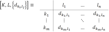
Then we can construct an index matrix

D =

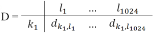
[K, L, \{d_{k_{i}, l_{j}}\}]

of probability trials:

where

d_{k_{i}, l_{j}}

= 1, if ωϵk_i and

d_{k_{i}, l_{j}}

= 0, if ω∉k_i, where 1 ≤ j ≤ n, 1 ≤ i ≤ m.

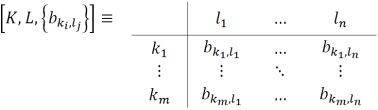
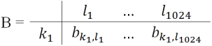
Analogously we can construct index matrix B =

[K, L, \{b_{k_{i}, l_{j}}\}]

of discrete random variables, where

b_{k_{i}, l_{j}}

is a predicate and denotes “

ω ϵ k_{i}

”.

5. Representation with IM a Value Read by Analog Pin of Arduino Uno Board

5.1. Definition of an Electrical Network

According to the definition, the electrical network is a combination of elements of interconnected circuits. The network may or may not provide a closed path to the flow of electricity. But an electrical circuit can be a combination of one or more networks that gives a closed path to the electric current. This means that when one or more networks are connected to each other to complete one or more current paths, an electrical circuit is formed. An electrical circuit consists of the following topological elements: node, branch and contour. A node is a point where two or more circuit topological elements are connected together. Node is a point of connection in the circuit. When a structural element of the circuit is connected to the circuit, it is connected through its two terminals to be part of a closed path. When a structural element exists between two nodes, the path from one node to another through this element is called a chain branch. If it starts from one node and after passing through a set of nodes returns to the same initial node without crossing two of the intermediate nodes, it travels through one node contour of the circuit.

[8, 9]

5.2. Embedded Systems and The Arduino Platform

An embedded system is an electronic circuit board that contains a microprocessor or microcontroller and other electronic parts, running a software program and used for a specific purpose rather than a general purpose as a Personal Computer(PC) would be used.

[7]

Arduino is composed of two major parts: an Arduino board and Arduino Integrated Development Environment(IDE). The Arduino board is a small microcontroller board, which is a small circuit (the board) that contains a whole computer on a small chip (the microcontroller)

[14].

In the years since the first Arduino was marketed, competitors have proliferated. Because of the large user base and the huge libraries of code that are available, Arduino boards are still very popular.

[11]

AVR microcontrollers, the microcontroller found on Arduino boards such as the Uno from Atmel are RISC microcontrollers that are available in 8-bit and 32-bit series.

[7]

The board, that we are going to use is Arduino Uno, because it is more widely used and it is possible shields to be added in the future.

[11]

5.3. Digital Pins of Arduino Uno

The digital pins of Arduino Uno define the input and output voltage level of the pins of the Breadboard. Also, the digital pins of Arduino Uno and the pins of the Breadboard forms a separate contour which activation depends entirely programmatically through the functions: digitalWrite (pin, value) and digitalRead (pin).

[8]

The function digitalRead() takes an argument of a given pin, either as a constant or variable. This will read in a value from a given pin and return either HIGH or LOW, this indicates either true/false, on/off, or 5 volts/0 volts. The function digitalWrite, which takes the arguments of a pin as well as HIGH or LOW, which will essentially turn a given pin on or off.

[15]

5.4. Analogread() function of Arduino

Analogread() function reads the value from the specified analog pin. Arduino boards contain a multichannel, 10-bit analog to digital converter. This means that it will map input voltages between 0 and the operating voltage (5 volts or 3.3 volts) into integer values between 0 and 1023. In contrast, the 10 bit SAR ADC reaches to the maximum code only after the input signal reaches the reference voltage level. As a result, the output code jumps from binary code 1022 to binary code 1024 while the input transitions from one subrange to the next.

[3]

On an Arduino UNO, for example, this yields a resolution between readings of: 5 volts / 1024 units or, 0.0049 volts per unit.

On ATmega based boards (UNO, Nano, Mini, Mega), it takes about 100 microseconds to read an analog input, so the maximum reading rate is about 10,000 times a second.

[4]

5.5. Application of an Index Matrix of Probability Trials and an Index Matrix of Discrete Random Variables with Arduino

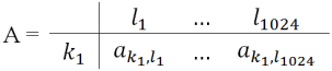
Let with X = {x₁, x₂, …, x₁₀₂₄ } integer values between 0 and 1023, where x₁ = 0, x₂ = 1, …, x₁₀₂₄ = 1023 and δ(x_j, x_j+1)=1, where 1 ≤ j ≤ 1023. Let with the index set L = {l₁, l₂, …, l₁₀₂₄ } denote intervals of 1024 units, where each unit is calculated by the function F(x_j) = l_j = x_j*(0.0049), where 1 ≤ j ≤ 1024.

From the Theorem, if there is a distribution function F(x), xϵR, then there exists a probability space (Ω, F, P) and a random variable ξ=ξ(ω), ωϵΩ with distribution function F(x).

Let with k₁ denote a value that has to be read by analog pin of Arduino Uno.

Then let

a_{k_{1}, l_{j}}

= F(x_j) = l_j = x_j*(0.0049),

where 1 ≤ j ≤ 1024. Then we can construct Index matrix

[k_{1}, L, \{a_{k_{1}, l_{j}}\}]

with elements

a_{k_{1}, l_{j}}

that are the results of calculations of function F(x_j) for each element x_j, where 1 ≤ j ≤ 1024.

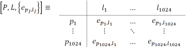
Let with each element of an index set P = { p₁, p₂, …, p₁₀₂₄)} denote each value of of function F(x_j) for each element x_j, where 1 ≤ j ≤ 1024, p₁=F(x₁), p₂=F(x₂), …, p₁₀₂₄=F(x₁₀₂₄).

Then we can construct Index matrix E=

[P, L, \{e_{p_{j}, l_{j}}\}]

with elements

e_{k_{1}, l_{j}}

that are the results of calculations of function F(x_j) for each element x_j, where 1 ≤ j ≤ 1024.

Let that value read the analog pin of Arduino Uno is 2.5 volts. Let we define a predicate with b. Let the predicate b denotes “F(x_j) <= 2.5 volts”.

Then we can construct Index matrix B =

[k_{1}, L, \{b_{k_{1}, l_{j}}\}]

of discrete random variables.

Let with ω₁ =

b_{k_{1}, l_{j}}

denote success and with ω₂ = ⌐

b_{k_{1}, l_{j}}

denote unsuccess, where 1 ≤ j ≤ 1024.

Then Ω = {ω₁, ω₂}.

Each Excel Workbook consists of pages named Worksheets, which are constructed by rows and columns forming cells.

[5, 6]

Let with the rows from 1 to 1024 of one Excel Sheet denote with the index set P and with an index set Q = {q₁, q₂} denote column A and column B of the same Excel Sheet. Then we can construct Index matrix H =

[P, Q, \{h_{p_{j}, q_{s}}\}]

, where the values of the elements (cells) of the first column q₁ (column A) and for each row consecutively of IM H and of the Excel Sheet will be the integer values from 0 to 1023 and the values of the elements (cells) of the second column q₂ (column B) and for each row consecutively of IM H and of the Excel Sheet will be the results of calculations of function F(x_j) for each element x_j, where 1 ≤ j ≤ 1024 and 1 ≤ s ≤ 2.

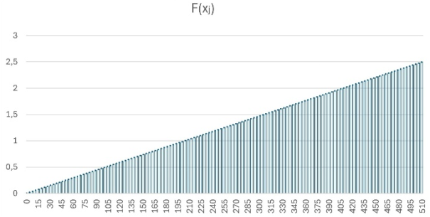
On figure 1 is illustrated a chart table that is generated from the values from cell A1 to cell B511, where the coordinates along the axis X

[5]

correspond to the indexes p₁, p₂, …, p₅₁₁of the index set P and the coordinates along the axis Y

[5]

correspond to the indexes l₁, l₂, …, l₅₁₁of the index set L of the Index matrix E. On figure 1 we can see that when x₅₁₁ =510 then the value calculated of function F(x₅₁₁) is less than 2.5.

Download: Download full-size image

Figure 1. Chart table, which illustrates the values of F(x_j) are less than 2.5, where j ≤ 511.

Let with the function

I_{k_{1} l_{j}}

(ω)=

\{\begin{matrix} 1 п ри ω ϵ k_{1} \\ 0 при ω \notin k_{1}, \end{matrix}

where

k_{1}

ϵ F, ωϵΩ define indicator of event k₁, where 1 ≤ j ≤ 1024.

Then we can construct Index matrix

D =

[k_{1}, L, \{d_{k_{1}, l_{j}}\}]

of probability trials.

6. Conclusions

In this article with the apparatus of Index Matrices were represented IM of probability trials and IM of discrete random variables. Illustrations with IMs, which elements are distribution functions, values read by analog pin of Arduino Uno board and probability trials were presented. A Chart table, which illustrates the values of distribution function F(x_j), which denotes a resolution between the readings by the analog pin of Arduino Uno board: 5 volts / 1024 units or 0.0049 volts per unit, where x₁, x₂, …, x₁₀₂₄ denote the points of discontinuity of F(l_j), are less than 2.5 volts for 1 ≤ j ≤ 511. According to the division of the number of desired outcomes by all numbers of outcomes can be calculated a relative frequency of the event in the case, when the points of discontinuity of F(l_j), are less than 2.5 volts for 1 ≤ j ≤ 511, which is a real number in the diapason [0,1]. In this way degrees of membership of desired outcomes and degrees of non-membership of not desired outcomes can be defined.

Abbreviations

IM	Index Matrix
L-IM	Logical IM

Author Contributions

Stela Todorova is the sole author. The author read and approved the final manuscript.

Conflicts of Interest

The author declares no conflicts of interest.

References

[1]	Atanassov, K. Index Matrices: Towards an Augmented Matrix Calculus. Springer, Cham (2014). https://doi.org/10.1007/978-3-319-10945-9
[2]	Димитров, М. Теория на вероятностите. Университетско издателство "Стопанство". София. 2002. [Dimitrov, M. Theory of probability. (2002) University Publishing House "Stopanstvo". Sofia]
[3]	Aksin, D., Al-Shyoukh, M. A., Maloberti, F. "An 11 Bit Sub Ranging SAR ADC with Input Signal Range of Twice Supply Voltage"; IEEE International Symposium on Circuits and Systems, ISCAS 2007, New Orleans, 27, 30 May 2007, pp. 1717-1720. https://doi.org/10.1109/ISCAS.2007.377925
[4]	Arduino. analogRead (). Available at https://www.arduino.cc/reference/tr/language/functions/analog-io/analogread/
[5]	Сотирова, Е. Димитрова, Л. Иновска, Г. Гордън, Г. Михайлова, Р. Илиева, П. Панайотов, Х. Мавров, Д. Ръководство за лабораторни упражнения по информатика. Бургас. 2013. [Sotirova, E. Dimitrova, L. Inovska, G. Gorden, G. Mihailova, R. Ilieva, P. Panayotov H. Mavrov, D. Guide to informatics laboratory exercises (2013) Burgas]
[6]	Todorova, S. Research of the index matrices and their applications. University "Prof. A. Zlatarov" (AU). Faculty of Technical Sciences. Academic degree: Doctor (PhD). 30.09.2024. Supervisor: Assoc. Prof. Veselina Kuncheva Bureva, PhD; Assoc. Prof. Nora Angelova Angelova, PhD. Reviewers: Acad. Prof. Krassimir Todorov Atanassov, DSc DSc Assoc. Prof. Velin Stoqanov Andonov, PhD. Burgas. 113 pages.
[7]	Smith W. A. C Programming with Arduino. Elektor International Media B. V. 2016.
[8]	Todorova, S. Proykov, M. Mathematical analysis of an electrical circuit. International Scientific Industry 4.0. Volume 6. Issue 1. pp. 25 26. 2021.
[9]	Riverglennapt, Nodes, branches and loops of a circuit, Available: https://riverglennapts.com/bg/circuit-and-network/172-nodes-branches-and-loops-of-a-circuit.html
[10]	Тодорова, С. Обзор върху публикациите по индексирани матрици. Годишник на секция "Инорматика". Съюз на учените в България. стр. 32 – стр. 62. Том XII. 2022-2023 [Todorova, S. Overview of publications on index matrices. (2022-2023) Yearbook of Section "Informatics". Union of Scientists in Bulgaria. pp. 32-62. Tom XII].
[11]	Platt, Ch. Make: Electronics: Learning by Discovery: A hands-on primer for the new electronics enthusiast. Third Edition. Published by Make Community, LLC. 2021.
[12]	Атанасов, К. Бурева В. Кратък курс по дискретни структури. Авангард Прима. гр. София. 2018 [Atanassov, K. Bureva V. Short course on discrete structures (2018). Avangard Prima. Sofia].
[13]	Birkhoff, G. Lattice Theory, Providence, RI: AMS, 1940.
[14]	Banzi, M. Shiloh M. Getting Started with Arduino: The Open Source Electronics Prototyping Platform. 4^th Edition. Published by Make Community, LLC. 2022.
[15]	Price, M. Arduino: 2 Books in 1: The Comprehensive Beginner's Guide to Take Control of Arduino Programming & Best Practices to Excel While Learning Arduino Programming. Publisher: ‎CreateSpace Independent Publishing Platform (May 18, 2018). 2018.
[16]	Todorova, S. Bureva, V. Angelova, N. Proykov M. Programme Product for Index Matrices. Book of Abstracts of International Symposium on Bioinformatics and Biomedicine 8-10 October 2020, Burgas, Bulgaria.

Cite This Article

Plain Text BibTeX RIS

APA Style

Todorova, S. (2025). Representation with Index Matrices Discrete Random Variables. American Journal of Applied Mathematics, 13(1), 57-63. https://doi.org/10.11648/j.ajam.20251301.14

Copy | Download

ACS Style

Todorova, S. Representation with Index Matrices Discrete Random Variables. Am. J. Appl. Math. 2025, 13(1), 57-63. doi: 10.11648/j.ajam.20251301.14

Copy | Download

AMA Style

Todorova S. Representation with Index Matrices Discrete Random Variables. Am J Appl Math. 2025;13(1):57-63. doi: 10.11648/j.ajam.20251301.14

Copy | Download

@article{10.11648/j.ajam.20251301.14,
  author = {Stela Todorova},
  title = {Representation with Index Matrices Discrete Random Variables},
  journal = {American Journal of Applied Mathematics},
  volume = {13},
  number = {1},
  pages = {57-63},
  doi = {10.11648/j.ajam.20251301.14},
  url = {https://doi.org/10.11648/j.ajam.20251301.14},
  eprint = {https://article.sciencepublishinggroup.com/pdf/10.11648.j.ajam.20251301.14},
  abstract = {With the Theory of probabilities it is made a mathematical description of a finite set of probability trials with random outcomes. Basically, the results from a given laboratory experiment are illustrated with tables, diagrams, ordinary matrices. Index matrices are a new approach of presenting and analyzing information of data. In this article the author will represent with Index Matrices, which elements are real numbers; function-type of elements, with which results of formulas with different parameters can be calculated and predicates, with which can be checked if a random outcome meets certain conditions according to a finite set of interval order. In order the data that we analyze to be more precisely verified, is not only ordered sequentially, but also a result of calculation of parameters from a given diapason at equal intervals. In this way the number of desired outcomes can be compared with not desired outcomes and with the data from different experiments, which can result in prediction of alternative values in the future. An illustration with Excel is described with an Index matrix, which elements are voltages between 0 and a value read by analog pin of Arduino Uno board, which is also presented with X and Y axis of a Chart diagram.},
 year = {2025}
}

Copy | Download

TY  - JOUR
T1  - Representation with Index Matrices Discrete Random Variables
AU  - Stela Todorova
Y1  - 2025/02/10
PY  - 2025
N1  - https://doi.org/10.11648/j.ajam.20251301.14
DO  - 10.11648/j.ajam.20251301.14
T2  - American Journal of Applied Mathematics
JF  - American Journal of Applied Mathematics
JO  - American Journal of Applied Mathematics
SP  - 57
EP  - 63
PB  - Science Publishing Group
SN  - 2330-006X
UR  - https://doi.org/10.11648/j.ajam.20251301.14
AB  - With the Theory of probabilities it is made a mathematical description of a finite set of probability trials with random outcomes. Basically, the results from a given laboratory experiment are illustrated with tables, diagrams, ordinary matrices. Index matrices are a new approach of presenting and analyzing information of data. In this article the author will represent with Index Matrices, which elements are real numbers; function-type of elements, with which results of formulas with different parameters can be calculated and predicates, with which can be checked if a random outcome meets certain conditions according to a finite set of interval order. In order the data that we analyze to be more precisely verified, is not only ordered sequentially, but also a result of calculation of parameters from a given diapason at equal intervals. In this way the number of desired outcomes can be compared with not desired outcomes and with the data from different experiments, which can result in prediction of alternative values in the future. An illustration with Excel is described with an Index matrix, which elements are voltages between 0 and a value read by analog pin of Arduino Uno board, which is also presented with X and Y axis of a Chart diagram.
VL  - 13
IS  - 1
ER  -

Copy | Download

Author Information

Stela Todorova

Department of Mathematics, Informatics and Physics, “Prof. Dr Assen Zlatarov” University, Burgas, Bulgaria

Biography: Stela Todorova is a Doctor of Technical sciences graduated at the University "Prof. Dr. Asen Zlatarov", Department “CST”, Faculty of Technical Sciences with the topic of her dissertation "Research of the index matrices and their applications". She graduated High School of Natural Sciences and Mathematics “Acad. Nikola Obreshkov”, Bachelor's degree in Informatics and Computer Science and Master's degree in Information Security at BFU, Burgas. Her current research interests are in the field of index matrices, intuitionistic fuzzy sets and etc.

Research Fields: Index Matrices, Fuzzy logic

Contact Email

http://orcid.org/0000-0002-0418-5853

Download PDF

Figure 1

Figure 1. Chart table, which illustrates the values of F(x_j) are less than 2.5, where j ≤ 511.

Plain Text BibTeX RIS

APA Style

Todorova, S. (2025). Representation with Index Matrices Discrete Random Variables. American Journal of Applied Mathematics, 13(1), 57-63. https://doi.org/10.11648/j.ajam.20251301.14

Copy | Download

ACS Style

Todorova, S. Representation with Index Matrices Discrete Random Variables. Am. J. Appl. Math. 2025, 13(1), 57-63. doi: 10.11648/j.ajam.20251301.14

Copy | Download

AMA Style

Todorova S. Representation with Index Matrices Discrete Random Variables. Am J Appl Math. 2025;13(1):57-63. doi: 10.11648/j.ajam.20251301.14

Copy | Download

@article{10.11648/j.ajam.20251301.14,
  author = {Stela Todorova},
  title = {Representation with Index Matrices Discrete Random Variables},
  journal = {American Journal of Applied Mathematics},
  volume = {13},
  number = {1},
  pages = {57-63},
  doi = {10.11648/j.ajam.20251301.14},
  url = {https://doi.org/10.11648/j.ajam.20251301.14},
  eprint = {https://article.sciencepublishinggroup.com/pdf/10.11648.j.ajam.20251301.14},
  abstract = {With the Theory of probabilities it is made a mathematical description of a finite set of probability trials with random outcomes. Basically, the results from a given laboratory experiment are illustrated with tables, diagrams, ordinary matrices. Index matrices are a new approach of presenting and analyzing information of data. In this article the author will represent with Index Matrices, which elements are real numbers; function-type of elements, with which results of formulas with different parameters can be calculated and predicates, with which can be checked if a random outcome meets certain conditions according to a finite set of interval order. In order the data that we analyze to be more precisely verified, is not only ordered sequentially, but also a result of calculation of parameters from a given diapason at equal intervals. In this way the number of desired outcomes can be compared with not desired outcomes and with the data from different experiments, which can result in prediction of alternative values in the future. An illustration with Excel is described with an Index matrix, which elements are voltages between 0 and a value read by analog pin of Arduino Uno board, which is also presented with X and Y axis of a Chart diagram.},
 year = {2025}
}

Copy | Download

TY  - JOUR
T1  - Representation with Index Matrices Discrete Random Variables
AU  - Stela Todorova
Y1  - 2025/02/10
PY  - 2025
N1  - https://doi.org/10.11648/j.ajam.20251301.14
DO  - 10.11648/j.ajam.20251301.14
T2  - American Journal of Applied Mathematics
JF  - American Journal of Applied Mathematics
JO  - American Journal of Applied Mathematics
SP  - 57
EP  - 63
PB  - Science Publishing Group
SN  - 2330-006X
UR  - https://doi.org/10.11648/j.ajam.20251301.14
AB  - With the Theory of probabilities it is made a mathematical description of a finite set of probability trials with random outcomes. Basically, the results from a given laboratory experiment are illustrated with tables, diagrams, ordinary matrices. Index matrices are a new approach of presenting and analyzing information of data. In this article the author will represent with Index Matrices, which elements are real numbers; function-type of elements, with which results of formulas with different parameters can be calculated and predicates, with which can be checked if a random outcome meets certain conditions according to a finite set of interval order. In order the data that we analyze to be more precisely verified, is not only ordered sequentially, but also a result of calculation of parameters from a given diapason at equal intervals. In this way the number of desired outcomes can be compared with not desired outcomes and with the data from different experiments, which can result in prediction of alternative values in the future. An illustration with Excel is described with an Index matrix, which elements are voltages between 0 and a value read by analog pin of Arduino Uno board, which is also presented with X and Y axis of a Chart diagram.
VL  - 13
IS  - 1
ER  -

Copy | Download