A Bayesian Spatial Deep Learning Framework for Mapping ZIP Code-Level Syphilis Hotspots in Hillsborough County, Florida

Aya Alhalbas; Salah-Eddin Komrokji; Aarya Preetam Satardekar; Rishil Shah; Namit Choudhari; James Jedrzejczyk; Benjamin Jacob

doi:doi:10.11648/j.ajai.20261002.15

Research Article |

A Bayesian Spatial Deep Learning Framework for Mapping ZIP Code-Level Syphilis Hotspots in Hillsborough County, Florida

Aya Alhalbas^*, Salah-Eddin Komrokji, Aarya Preetam Satardekar, Rishil Shah, Namit Choudhari, James Jedrzejczyk, Benjamin Jacob

Published in American Journal of Artificial Intelligence (Volume 10, Issue 2)

Received: 6 July 2026 Accepted: 8 August 2026 Published: 15 September 2026

Views: Downloads:

Download PDF

Share This Article

Twitter
Linked In
Facebook

Abstract

Syphilis has re-emerged as a major public health concern in the United States, exhibiting substantial spatial heterogeneity that is inadequately captured by conventional surveillance systems. This study presents an integrated spatial-statistical and deep learning framework to identify ZIP Code Tabulation Area (ZCTA)-level syphilis hotspots in Hillsborough County, Florida, by combining epidemiological surveillance data, socioeconomic and racial covariates, and Sentinel-2 satellite-derived environmental indicators. Syphilis incidence was modeled using a Poisson generalized linear model with population offsets, while spatial dependence was addressed using a Bayesian hierarchical Conditional Autoregressive (CAR) model within the Besag-York-Mollie (BYM) framework. We further introduce an eigen-Bayesian convolutional neural network (EBCNN) that incorporated eigen-decomposition of spatial weight covariance matrices, enabling spectral regularization and improved representation of latent spatial autocorrelation in the upscaled sampled ZCTA georeferenced capture point data. Sentinel-2 Level-2A imagery was used to derive environmental predictors, including the Normalized Difference Vegetation Index (NDVI) and Normalized Difference Built-up Index (NDBI), aggregated to ZCTAs through zonal statistics. Random Forest (RF), Support Vector Machine (SVM), and Gradient Boosting Tree classifiers were trained to distinguish high- and low-risk ZCTAs. Model performance was evaluated using cross-validation, area under the receiver operating characteristic curve (AUC), sensitivity, and specificity. Results indicate that higher syphilis incidence is significantly associated with socioeconomic deprivation, increased urban density, and reduced vegetation cover. Incorporating spatial random effects reduced residual spatial autocorrelation and improved hotspot stability in ZIP Codes. Global Moran's I = 0.34, p < 0.001. Following implementation of the Besag-York-Mollie (BYM) spatial model, Moran's I decreased to 0.07 (p = 0.18). The proposed EBCNN achieved superior hotspot detection accuracy and uncertainty calibration compared with conventional deep learning models. Integrating satellite-derived environmental variables with demographic and socioeconomic factors provides a scalable, high-resolution framework for precision public health surveillance and targeting potential syphilis ZCTA vulnerable populations for interventions.

Published in	American Journal of Artificial Intelligence (Volume 10, Issue 2)
DOI	10.11648/j.ajai.20261002.15
Page(s)	219-235
Creative Commons	This is an Open Access article, distributed under the terms of the Creative Commons Attribution 4.0 International License (http://creativecommons.org/licenses/by/4.0/), which permits unrestricted use, distribution and reproduction in any medium or format, provided the original work is properly cited.
Copyright	Copyright © The Author(s), 2026. Published by Science Publishing Group

Keywords

Syphilis, Sentinel-2, Random Forest, Support Vector Machine, Gradient Boosting Trees, Bayesian CAR Model, Eigen-Bayesian Convolutional Neural Network, ZIP Code Hotspots

1. Introduction

Sexually transmitted infections (STIs) remain a persistent public health challenge in the United States, with syphilis rates increasing markedly over the past decade. After reaching historic lows in the early 2000s, syphilis has re-emerged as a major concern, particularly among urban populations and socioeconomically marginalized communities. According to the Centers for Disease Control and Prevention (CDC), reported cases of primary and secondary syphilis increased by more than 700% between 2000 and 2023, with over 176,000 total syphilis cases reported in 2023 alone in the United States, including more than 53,000 primary and secondary infections, the most infectious stages of the disease Centers for Disease Control and Prevention

[9]

https://www.cdc.gov/std/statistics. Congenital syphilis has also risen sharply, with over 3,700 reported cases in 2022, representing a more than tenfold increase over the past decade.

[9]

These trends underscore a sustained and worsening epidemic, particularly concentrated in southeastern states such as Florida, which consistently ranks among the highest-burden jurisdictions for syphilis incidence.

In Florida, syphilis transmission exhibits strong spatial heterogeneity at sub-county scales, with urban centers such as Tampa (Hillsborough County) demonstrating pronounced clustering of cases. Hillsborough County is among the state’s highest-burden areas, with persistent increases in primary and secondary syphilis rates over the past decade, particularly in neighborhoods characterized by socioeconomic deprivation, housing instability, and high population mobility

[18]

. These fine-scale disparities highlight the limitations of conventional surveillance systems, which typically report incidence at the county level, thereby masking localized transmission dynamics that are essential for targeted intervention.

Understanding the spatial distribution of syphilis at granular geographic levels is therefore critical for precision public health interventions. Traditional epidemiological approaches rely on aggregated surveillance data and generalized linear models that often fail to capture spatial dependence and unobserved heterogeneity. To address these limitations, spatial statistical frameworks such as the Besag-York-Mollie (BYM) model and Conditional Autoregressive (CAR) priors have been widely adopted for disease mapping, allowing explicit modeling of spatial autocorrelation in areal data

[4, 31]

. However, these models remain limited in their ability to integrate high-dimensional nonlinear covariates such as remote sensing imagery.

Recent advances in geospatial artificial intelligence (Geo-AI) and deep learning have introduced convolutional neural networks (CNNs) as powerful tools for extracting spatial representations from satellite imagery. Bayesian convolutional neural networks (BCNNs) extend standard CNNs by incorporating probabilistic weight distributions, enabling uncertainty-aware spatial prediction

[20, 26, 27]

. Building on these developments, this study employs an eigen-Bayesian convolutional neural network (EBCNN) framework, which integrates spectral decomposition of spatial feature covariance structures into a Bayesian deep learning architecture. Attention-based representation learning provides an additional mechanism for emphasizing informative features within high-dimensional neural architectures

[43]

. The eigen-decomposition step projects learned convolutional feature maps onto a low-dimensional orthogonal basis derived from the graph Laplacian of spatial adjacency structures, consistent with spectral graph theory and Laplacian eigenmaps

[3]

. Graph-based neural approaches provide a framework for representing relationships among spatially connected units and learning from their underlying neighborhood structure

[49]

. We assumed that this formulation would enhance a stratified upscaled syphilis vulnerable population hotspot model’s ability to explicitly encode spatial autocorrelation, multi-scale geographic structure, and nonstationary neighborhood effects.

Within this EBCNN framework, Sentinel-2 Level-2A multispectral imagery was employed to derive environmental and built-environment indicators, including normalized difference vegetation index (NDVI), normalized difference built-up index (NDBI), and other land-cover proxies. These features were aggregated to ZIP Code Tabulation Areas (ZCTAs) using zonal statistics, enabling integration with sociodemographic, racial, and socioeconomic covariates derived from U.S. Census Bureau datasets. Remote sensing variables are increasingly recognized as valid proxies for structural determinants of health, including urban density, land use heterogeneity, and environmental deprivation

[30, 50]

In parallel, supervised machine learning methods, including Random Forests (RFs), Support Vector Machines (SVMs), and Gradient Boosting Trees (GBT), were employed for classification of high- and low-risk syphilis burden ZCTAs. These ensemble learning approaches have demonstrated strong performance in epidemiological prediction tasks due to their ability to model nonlinear interactions and high-dimensional feature spaces

[7, 19]

. Recent studies have shown their effectiveness in STI risk prediction, including HIV, gonorrhea, and chlamydia classification using clinical and behavioral datasets, where GBT and RF methods consistently outperform traditional regression-based models

[2, 25, 40]

Our assumption was that EBCNN could integrate Sentinel-2-derived environmental features with graph-based spectral representations of Laplacian eigenmaps encoding spatial connectivity among neighboring ZCTA hot spots, enabling the network to learn multi-scale spatial dependencies while Bayesian inference quantifies predictive uncertainty. This framework hence would produce high-resolution probabilistic hotspot maps that identify ZIP code-level syphilis risk by jointly modeling environmental, demographic, socioeconomic, and spatial drivers of disease transmission.

Syphilis mapping is essential for identifying transmission hotspots and guiding targeted public health interventions. However, existing CDC and state-level surveillance systems typically report aggregated incidence data that are insufficient for ZIP code-level decision-making. Although valuable, these coarse-resolution datasets do not capture micro-scale heterogeneity in transmission risk, limiting their utility for precision intervention design

[9]

Given the severe consequences of untreated syphilis, including congenital syphilis, neurological complications, and increased HIV transmission risk, there is currently a critical need for high-resolution predictive modeling frameworks

[27, 29, 42]

. This study therefore integrates epidemiological surveillance data, Sentinel-2 remote sensing indicators, and socioeconomic covariates within a unified machine learning and Eigen-BCNN framework to model syphilis risk at the ZCTA level in Hillsborough County, Florida.

The hypotheses in this experiment were:

H1: Sentinel-2-derived environmental and built-environment indicators contain statistically significant spatial information associated with ZIP code-level syphilis burden.

H2: Machine learning models and EBCNN can integrate multisource geospatial and demographic data for accurate hotspot detection at the ZCTA level.

H3: Ensemble learning methods (RF, GBTs) and EBCNN models will outperform SVMs due to improved representation of nonlinear and spatially autocorrelated processes.

H4: Urbanization, land-cover heterogeneity, socioeconomic deprivation, and racial/ethnic composition will emerge as dominant predictors of syphilis hotspot formation.

This study develops and evaluates a hybrid spatial-machine learning framework for predicting ZIP code-level syphilis hotspots in Hillsborough County, Florida. The specific aims are:

1) To derive Sentinel-2-based environmental and built-environment indicators (e.g., NDVI, NDBI) characterizing urban structure and ecological variation.

2) To integrate remote sensing features with ZIP code-level sociodemographic, socioeconomic, and racial covariates.

3) To develop and compare RF, SVM, GBTrees, and EBCNN models for syphilis risk classification.

4) To evaluate predictive performance using cross-validation and metrics including AUC, accuracy, sensitivity, specificity, and F1-score.

5) To quantify feature importance and spatial effects using permutation importance, partial dependence, and eigen-spatial saliency analysis within the EBCNN framework.

6) To generate high-resolution georeferenced ZIP code-level risk maps for precision public health surveillance and targeted intervention planning.

2. Materials and Methodology

2.1. Study Site

Hillsborough County is in the west-central portion of the U.S. state of Florida. In the 2020 census, the population was 1,459,762, making it the fourth-most populous county in Florida and the most populous county outside the Miami metropolitan area. An estimate in 2021 shows the population of Hillsborough County at 1,512,070 people, with a yearly growth rate of 1.34%, which itself is greater than the populations of 12 states according to their 2019 population estimates. Its county seat and largest city is Tampa. Hillsborough County is part of the Tampa-St. Petersburg-Clearwater Metropolitan Statistical Area (U.S. Census Bureau. (2021). Population Estimates Program: Hillsborough County, Florida population estimates).

2.2. Hillsborough County Study Site

Download: Download full-size image

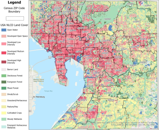
Figure 1. Map of Hillsborough County ZIP Code boundaries and land cover classifications.

2.3. Satellite Data

Sentinel-2 Level-2A imagery covering Hillsborough County, Florida, was acquired from the European Space Agency (ESA) Copernicus Open Access Hub and processed using a custom Python-based geospatial workflow. Multispectral remote-sensing imagery can be processed and classified to characterize land-cover and built-environment features

[24]

. Sentinel-2 is a multispectral Earth observation mission consisting of twin satellites (Sentinel-2A and Sentinel-2B) that provide varying moderate resolution spatial resolution imagery with 13 spectral bands for environmental monitoring and land-cover mapping (Table 1). All Sentinel-2 tiles intersecting the study area were downloaded and screened using scene metadata to verify acquisition dates, cloud coverage percentages, and geometric quality.

To minimize atmospheric and cloud-related contamination, only Sentinel-2 Level-2A scenes with less than 10% cloud cover were retained for analysis. Level-2A products provide bottom-of-atmosphere (BOA) surface reflectance generated through the Sen2Cor atmospheric correction algorithm, ensuring radiometrically consistent observations suitable for quantitative spectral analyses

[33]

Cloud and shadow contamination were identified using the Sentinel-2 Scene Classification Layer (SCL), which classified pixels into categories including urban, peri-urban rural farmland. Pixels were classified using a binary cloud mask implemented in Python. Image preprocessing, which was performed using Rasterio, NumPy, and GeoPandas libraries. These were used to read raster datasets, generate cloud masks, and remove contaminated pixels before spectral analysis.

The spatial extent of the imagery was subsequently restricted to the study region using a Hillsborough County boundary shapefile obtained from local GIS resources. All Sentinel-2 scenes were projected into Universal Transverse Mercator (UTM) Zone 17 North (EPSG: 32617), the recommended coordinate reference system for regional analyses in west-central Florida. Raster datasets were clipped to the county boundary using masking functions implemented in Python with the Rasterio and GeoPandas libraries.

2.4. Topographic Landscape Maps

A land-use/land-cover (LULC) map of Hillsborough County, Florida, was developed using multispectral Sentinel-2 Level-2A imagery with a spatial resolution of 10 m. Image processing was conducted in Python using the Rasterio, GeoPandas, NumPy, xarray, rioxarray, SentinelHub, and scikit-learn libraries. Four Sentinel-2 bands with 10-m spatial resolution were utilized: Blue (Band 2, 490 nm), Green (Band 3, 560 nm), Red (Band 4, 665 nm), and NIR (Band 8, 842 nm). Sentinel-2 spectral bands provide sufficient information for distinguishing urban surfaces, vegetation, water bodies, wetlands, and agricultural land cover

[39, 46]

Training samples representing urban surfaces (dense buildings and roads in central Hillsborough County), peri-urban transition zones with mixed housing and vegetation, and rural farmland dominated by cropland and smallholder fields were collected from high-resolution reference imagery using georeferenced, capture-point-sampled online data. A supervised classification algorithm (i.e., maximum likelihood) was applied to classify the stacked spectral bands and indices into the three land-cover categories.

To characterize environmental conditions and built-environment features potentially associated with syphilis transmission, spectral indices were derived from atmospherically corrected Sentinel-2 Level-2A surface reflectance imagery using a custom Python-based geospatial processing workflow. Spectral indices provide quantitative measures of vegetation abundance, urban development intensity, and landscape heterogeneity and have been widely employed in environmental health and spatial epidemiology studies

[37, 51]

The Normalized Difference Vegetation Index (NDVI) was calculated to quantify vegetation density and photosynthetic activity throughout Hillsborough County. NDVI exploits the strong reflectance contrast between the red and near-infrared regions of the electromagnetic spectrum, which was computed using Sentinel-2 Band 8 (Near Infrared, 842 nm) and Band 4 (Red, 665 nm) as:

NDVI = \frac{NIR - Red}{NIR + Red}

where:

1) NIR = Near-Infrared band

2) Red = Red band

Typical interpretation:

1) +0.6 to +1.0: Dense, healthy vegetation

2) +0.2 to +0.5: Sparse vegetation or crops

3) 0 to +0.2: Bare soil

4) < 0: Water, clouds, or built-up surfaces

We also generated an Normalized Difference Built-up Index (NDBI) to identify built-up or urban areas.

NDBI = \frac{SWIR - NIR}{SWIR + NIR}

where:

1) SWIR = Shortwave Infrared band

2) NIR = Near-Infrared band

Interpretation:

1) Positive values: Built-up or urban areas

2) Around 0: Mixed land cover

3) Negative values: Vegetation or water

Band combinations included:

Table 1. Sentinel-2 Spectral Bands Used for NDVI and NDBI.

Satellite:	Red	NIR	SWIR (used for NDBI)
Sentinel-2 MSI	Band 4	Band 8	Band 11 (SWIR1)

1) Sentinel-2

2) NDVI = (Band 8 − Band 4) / (Band 8 + Band 4)

3) NDBI = (Band 11 − Band 8) / (Band 11 + Band 8)

NIR denotes surface reflectance in Sentinel-2 Band 8, and Red denotes surface reflectance in Sentinel-2 Band 4 data [https://sentinels.copernicus.eu/copernicus/sentinel-2]. NDVI values theoretically range from -1 to +1, with values approaching +1 indicating dense healthy vegetation, values near zero representing bare soil or sparsely vegetated surfaces, and negative values generally corresponding to water bodies or non-vegetated surfaces

[37, 41]

All proxy spectral indices were computed from cloud-masked Sentinel-2 imagery using custom Python scripts implemented with NumPy, Rasterio, and GeoPandas libraries. Following index generation, zonal statistical summaries were calculated for each ZCTA using GIS-based spatial aggregation procedures. Specifically, the mean, median, standard deviation, minimum, and maximum NDVI and NDBI values were extracted for each ZCTA and subsequently used as predictor variables in the machine-learning classification framework. These remotely sensed environmental indicators were analyzed jointly with sociodemographic, racial, and socioeconomic covariates to improve the detection and prediction of ZIP code-level syphilis hotspots throughout Hillsborough County, Florida.

2.5. Zip Codes and Vulnerability Indices

Probabilities from population-stratified demographic, socioeconomic, and racial, non-time series sampled covariates were acquired from the United States Census Bureau (2020) for Hillsborough County. The vulnerability indices included ZCTA stratification for county-level incidence of syphilis which was retrieved from publicly available Florida Department of Health surveillance data The number of syphilis cases for each zip code was calculated by cross-multiplying the estimated total cases for the county from the Point-in-Time count (2025) using the ratio of male and female cases from the count the year before (Point-in-Time, 2024) and the population for each zip code. This had to be performed since the data for syphilis cases at a zip code level was unavailable, and gender statistics for the homeless population were not made publicly available for the 2025 count.

Incidence rate at the ZCTA level was calculated as the number of reported cases per population. Counts of reported syphilis cases were obtained from surveillance data and paired with corresponding population denominators. Independent variables included epidemiologic ZCTA-level stratified racial, demographic, and socioeconomic characteristics derived from publicly available census data sources. These variables included, but were not limited to, racial/ethnic composition, median household income, educational attainment, employment status, housing characteristics, and population density. All covariates were standardized prior to analysis to facilitate model convergence and interpretation.

2.6. Spectral Interpolation and Machine Learning-Based Spatial Downscaling

Spectral interpolation was formulated as a change-of-support and latent Gaussian spatial process problem

[35]

, in which ZCTA-level syphilis observations are treated as noisy realizations of an underlying continuous spatial process. Following classical geostatistical theory

[11, 13]

, we let

y (s_{i})

denote the observed syphilis intensity at a spatial ZCTA-stratified location

s_{i} \in D \subset R^{2}

. The data-generating process was defined as:

y (s_{i}) = Z (s_{i}) + ε_{i}, ε_{i} \sim N (0, σ^{2})

where

Z (s)

was an unobserved latent spatial field representing true disease intensity.

The latent field was expressed using a spectral basis function decomposition, consistent with eigenfunction spatial filtering and low-rank spatial process representations

[16]

Z (s) = \sum_{k = 1}^{K} α_{k} ϕ_{k} (s)

where:

ϕ_{k} (s)

were orthogonal eigenfunctions of a spatial operator i.e., the Laplace-Beltrami

α_{k}

were unknown coefficients,

K ≪ n

ensures dimensionality reduction.

Eigenfunctions satisfy:

Δ ϕ_{k} (s) = λ_{k} ϕ_{k} (s)

where

Δ

was the Laplacian operator and

λ_{k}

are eigenvalues controlling spatial smoothness. This formulation is consistent with spectral spatial filtering approaches

[21]

and Gaussian process approximations using basis expansions

[13]

Coefficients were estimated using penalized least squares:

\hat{α} = \arg \min_{α} [∥ y - Φ α ∥^{2} + λ α^{T} Ω α]

where:

Φ_{ik} = ϕ_{k} (s_{i})

Ω

is a roughness penalty matrix

λ

controls spatial smoothness

This corresponded to a regularized inverse problem ensuring stable reconstruction of spatial fields.

To convert from capture point/ZCTA support to areal-level estimates (county level), the reconstructed field was integrated:

\hat{Z} (C_{j}) = \frac{1}{∣ C_{j} ∣} \int_{C_{j}} \hat{Z} (s) ds

In computational implementation, this was approximated using fine-resolution discretization:

\hat{Z} (C_{j}) \approx \frac{1}{∣ C_{j} ∣} \sum_{r \in R_{j}} w_{r} \hat{Z} (s_{r})

where:

R_{j}

are raster cells within county

C_{j}

w_{r}

are area weights

This follows standard change-of-support theory in spatial statistics

[12]

To incorporate nonlinear interactions between socioeconomic, racial, and demographic environmental predictors, supervised learning models were employed. We let

X_{i} \in R^{p}

denote the sampled covariates at ZCTA

i

. The general learning objective was:

\hat{f} = a rg \min_{f} \sum_{i = 1}^{n} L (y_{i}, f (X_{i})) + Ω (f) .

Random Forest was constructed using

\hat{f} (x) = \frac{1}{B} \sum_{b = 1}^{B} T_{b} (x) .

Each tree minimized node impurity using

G = 1 - \sum_{k} p_{k}^{2 .}

Gradient Boosting Machine i.e,

f_{m} (x) = f_{m - 1} (x) + η h_{m} (x)

generated weak learners that fit negative gradients:

h_{m} (x) \approx - [\frac{\partial L (y, f (x))}{\partial f (x)}] An XGBoost

objective function:

L = \sum_{i = 1}^{n} l (y_{i}, {\hat{y}}_{i}) + \sum_{k} Ω (f_{k})

was converted into a regularization term:

Ω (f) = γT + \frac{1}{2} λ ∥ w ∥^{2}

The SVM formulation was

\min_{w, b, ξ} \frac{1}{2} ∥ w ∥^{2} + C \sum_{i} ξ_{i}

which was subject to:

y_{i} (w^{T} x_{i} + b) \geq 1 - ξ_{i}

. The Kernel form:

K (x_{i}, x_{j}) = ϕ (x_{i})^{T} ϕ (x_{j})

was infused. The final hybrid estimator combined spectral reconstruction and machine learning prediction and generated:

\hat{Y} (s) = \underset{spectral spatial field}{\underset{⏟}{\sum_{k = 1}^{K} α_{k} ϕ_{k} (s)}} + \underset{nonlinear covariate effects}{\underset{⏟}{f_{ML} (X (s))}}

The spectral interpolation and machine learning framework was implemented entirely in Python using an open-source geospatial and machine learning environment. Data processing, spatial analysis, spectral index generation, and predictive modeling were conducted using Python version 3.11 within a Jupyter Notebook workflow to ensure reproducibility and transparency.

2.7. Statistical Modeling

A Poisson regression model was employed as the primary inferential framework to evaluate associations between syphilis incidence and socioeconomic, demographic, and remotely sensed environmental covariates across ZCTAs in Hillsborough County, Florida. Count-based regression models provide an appropriate framework for analyzing disease-event counts and incidence data

[8]

. This approach is widely used in infectious disease epidemiology for modeling rare count outcomes under varying population exposure

[31, 45]

. We let

Y_{i}

denote the observed number of syphilis cases in ZCTA

i

, assumed to follow a Poisson distribution:

Y_{i} \sim Poisson (λ_{i})

where

λ_{i}

is the expected number of cases.

Log-linear model specifications were generated. The generalized linear model (GLM) was defined as:

\log (λ_{i}) = β_{0} + \sum_{k = 1}^{p} β_{k} X_{ki} + \log (Po p_{i})

where:

X_{ki}

= covariates (socioeconomic, demographic, racial, environmental)

Po p_{i}

= population offset

β_{k}

= regression coefficients

The offset ensured that the model estimated incidence rates rather than raw counts. A likelihood function (Poisson GLM foundation) for the ZCTA stratified observations

was

constructed using:

P (Y_{i} = y_{i} ∣ λ_{i}) = \frac{λ_{i}^{y_{i}} e^{- λ_{i}}}{y_{i}!}

The full log-likelihood was:

L (β) = \sum_{i = 1}^{n} [y_{i} \log (λ_{i}) - λ_{i} - \log (y_{i}!)]

. Substituting the log-linear model:

λ_{i} = \exp (X_{i} β + \log (Po p_{i}))

generated

L (β) = \sum_{i = 1}^{n} [y_{i} (X_{i} β + \log (Po p_{i})) - \exp (X_{i} β + \log (Po p_{i})) - \log (y_{i}!)]

Parameter estimation (Maximum Likelihood Algorithm) was determined. Parameters were estimated using Iteratively Reweighted Least Squares (IRLS), standard for Poisson GLMs. We employed IRLS to Initialize

β^{(0)}

. Thereafter we iterated

t

using:

μ_{i}^{(t)} = \exp (X_{i} β^{(t)})

W_{i}^{(t)} = μ_{i}^{(t)}

z_{i}^{(t)} = X_{i} β^{(t)} + \frac{y_{i} - μ_{i}^{(t)}}{μ_{i}^{(t)}}

The formulation was updated using

β^{(t+ 1)} = (X^{T} WX)^{- 1} X^{T} Wz

This was repeated until convergence:

∣ β^{(t+ 1)} - β^{(t)} ∣ < ϵ

Model coefficients were interpreted using

IR R_{k} = e^{β_{k}}

which we assumed would represent the multiplicative change in syphilis incidence associated with a one-unit increase in covariate

X_{k}

, holding other variables constant.

2.8. Spatial Autocorrelation Diagnostics

Residual spatial dependence was assessed using Moran’s I:

I = \frac{n}{S_{0}} \frac{\sum_{i} \sum_{j} w_{ij} (e_{i} - \overset{̀}{e}) (e_{j} - \overset{̀}{e})}{\sum_{i} (e_{i} - \overset{̀}{e})^{2}}

where:

w_{ij}

= spatial weights matrix

e_{i}

= model residuals

Significant Moran’s I indicate spatial structure not captured by covariates

[21]

2.9. Bayesian Spatial Extension Framework

To account for spatial dependence, a Conditional Autoregressive (CAR) structure was defined:

u_{i} ∣ u_{- i} \sim N (\frac{\sum_{j \in N (i)} w_{ij} u_{j}}{\sum_{j \in N (i)} w_{ij}}, \frac{1}{τ_{u} \sum_{j \in N (i)} w_{ij}})

The full Besag-York-Mollie (BYM) model was:

\log (λ_{i}) = X_{i} β + u_{i} + v_{i} + \log (Po p_{i})

where:

u_{i}

: spatially structured effect

v_{i} \sim N (0, τ_{v}^{- 1})

: unstructured noise

Model performance was evaluated using:

1) Akaike Information Criterion (AIC):

AIC = - 2 L + 2 k

2) Deviance:

D = 2 (L_{sat} - L_{model})

3) Residual spatial autocorrelation (Moran’s I)

4) Pearson residual plots

Final model estimates were reported as incidence rate ratios (IRRs) with 95% confidence intervals:

CI = e^{β_{k} \pm 1.96 \cdot SE (β_{k})}

We defined an adjacency graph using

G = (V, E), A_{ij} = w_{ij}

A Graph Laplacian:

L = D - A

. We performed an eigen-decomposition:

L = U Λ U^{⊤}

where:

U

= eigenvectors (spatial basis functions),

Λ

= eigenvalues (spatial frequencies).

Eigen-Spectral Projection Input feature maps

X

were projected using

\tilde{X} = U^{⊤} X

. This transformed spatial signals into orthogonal eigen-space components.

A Standard convolution

Y = W * X + b

was generated. We used Bayesian formulation:

W \sim N (μ_{W}, Σ_{W})

. Posterior inference via variational approximation was generated

q (W) \approx p (W ∣ D)

with ELBO:

L_{ELBO} = E_{q (W)} [\log p (Y ∣ X, W)] - KL (q (W) ∥ p (W))

An Eigen-Bayesian Convolution was conducted in eigen-space using

Y = U \cdot g_{θ} (U^{⊤} X)

where

g_{θ}

was a Bayesian neural operator.

Eigen-Weights were generated using

α_{k} = \frac{\exp (λ_{k})}{\sum_{j} \exp (λ_{j})}

/. The final representation was

Z = \sum_{k} α_{k} U_{k}^{⊤} X .

The Predictive Distribution was determined using

p (y^{*} ∣ x^{*}, D) = \int p (y^{*} ∣ x^{*}, W) p (W ∣ D) dW

which was approximated via Monte Carlo sampling using

\hat{y} = \frac{1}{S} \sum_{s = 1}^{S} f_{W_{s}} (x^{*})

Model evaluation classification metrics were conducted using;

Accuracy = \frac{TP + TN}{TP + TN + FP + FN}

Sensitivity = \frac{TP}{TP + FN}

Specificity = \frac{TN}{TN + FP}

F 1 = 2 \cdot \frac{Precision \cdot Recall}{Precision + Recall}

ROC-AUC was then computed using

AUC = \int_{0}^{1} TPR (FP R^{- 1} (t)) dt

. For Cross-Validation (CV) we used K-fold:

CV = \frac{1}{K} \sum_{k = 1}^{K} L_{k}

The integrated multiscale model framework

Combined

F = \underset{spatial smoothing}{\underset{⏟}{BYM-CAR}} + \underset{nonlinear tabular learning}{\underset{⏟}{ML ensemble}} + \underset{spectral deep spatial learning}{\underset{⏟}{Eigen-BCNN}}

We assumed that these estimates could quantify the independent contribution of stratified socioeconomic, racial, and demographic predictors to vulnerable syphilis ZCTA populations while adjusting for spatial dependence. The final risk stratified estimate was quantified using:

{\hat{y}}_{i} = σ (f_{RF / SVM / GBT} (X_{i}) + f_{Eigen - BCNN} (z_{i}) + u_{i} + v_{i})

3. Results

Following preprocessing, the four Sentinel-2 spectral bands available at 10-m spatial resolution—Blue (Band 2; 490 nm), Green (Band 3; 560 nm), Red (Band 4; 665 nm), and Near-Infrared (Band 8; 842 nm) were stacked into a single multiband raster dataset. Digital number values were converted to surface reflectance by applying the Sentinel-2 scaling factor and dividing pixel values by 10,000 according to ESA product specifications

[17]

. The resulting cloud-free, georeferenced, and radiometrically standardized imagery served as the foundation for deriving vegetation indices, built-environment indicators, and land-use/land-cover variables used in subsequent machine-learning analyses for mapping ZCTA-level syphilis hotspots. All datasets were harmonized to the ZCTA level to ensure consistency across racial/ethnic, socioeconomic demographic remotely sensed variables.

All image processing, preprocessing, feature extraction, and LULC classification procedures were implemented through a custom Python workflow developed specifically for this study. The workflow utilized open-source geospatial and machine-learning libraries, including Rasterio, GeoPandas, NumPy, Xarray, Rioxarray, and Scikit-learn, to automate data ingestion, cloud masking, image mosaicking, spectral index computation, supervised classification, and accuracy assessment. The use of a scripted workflow ensured methodological consistency, computational reproducibility, and efficient processing of large Sentinel-2 datasets across the study area.

The final cloud-free Level-2A surface reflectance mapping data covered the Hillsborough County metropolitan region and surrounding peri-urban agricultural landscape. The key 10-m bands blue (B2), green (B3), red (B4), and near-[IR] (B8) were stacked and preprocessed with atmospheric correction, cloud masking, and clipping to the study boundary.

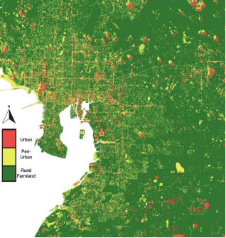
After classification, accuracy assessment using validation points evaluated the reliability of the map, and post-processing (such as smoothing and removing isolated pixels) we produced a final 10-m resolution land-use map distinguishing urban, peri-urban, and rural farmland zones. The LULC-classified map revealed the capture point, surface area (m²) of each, georeferenced, sentinel site, stratified, syphilis-related capture point population vulnerability site. (Figure 2).

Download: Download full-size image

Figure 2. LULC Hillsborough County Study Site Map.

The supervised LULC classification derived from Sentinel-2 10-m spatial resolution imagery demonstrated clear differentiation of urban, peri-urban, and rural farmland classes across Hillsborough County at the ZCTA level prior to spatial visualization. Classification outputs indicated substantial heterogeneity in land-use composition, reflecting the complex transition between densely developed metropolitan areas and surrounding agricultural and semi-natural landscapes.

Urban land cover was predominantly concentrated within central and highly developed ZCTAs, characterized by continuous impervious surfaces, transportation corridors, and commercial infrastructure. These areas exhibited high classification consistency, with low intra-zone variability, indicating homogeneous built-up environments. Several ZCTAs had a dominant proportion of urban pixels, suggesting strong clustering of development intensity in core metropolitan areas.

Peri-urban zones represented transitional landscapes and exhibited the highest degree of heterogeneity among the three classes. These areas were characterized by a mosaic of residential developments, fragmented vegetation, and small-scale land uses. ZCTAs classified as peri-urban displayed moderate variability in class proportions, reflecting mixed land-use patterns and ongoing urban expansion. This class frequently occurred at the interface between highly urbanized cores and outlying agricultural regions, indicating dynamic land transformation processes.

Rural farmland classification was primarily observed in peripheral ZCTAs and areas with lower population density, where agricultural land use and open spaces dominated. These zones exhibited relatively high classification uniformity, with large contiguous patches of farmland identified across multiple ZCTAs. The proportion of rural farmland was highest in eastern and southern portions of the county, consistent with known agricultural land distribution patterns.

Zonal aggregation of LULC classes revealed meaningful gradients in land-use composition across ZCTAs. The proportion of urban, peri-urban, and rural farmland pixels within each zone was quantified and incorporated as categorical and proportional predictors in the machine-learning classification framework. Preliminary model outputs suggested that ZCTAs with higher proportions of urban and peri-urban land cover were more strongly associated with elevated classification risk profiles, while rural farmland-dominated areas exhibited comparatively lower predicted risk.

Overall, prior to map visualization, the LULC classification results demonstrated that Sentinel-2-derived 10-m land cover data effectively capture spatial patterns of urbanization and landscape transition. These outputs provided a valuable representation of built-environment structure and land-use gradients.

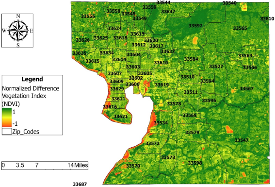
Descriptive analysis of spectral indices derived from Sentinel-2 imagery revealed substantial spatial variability in vegetation cover and built-environment intensity across Hillsborough County at ZCTA level. Prior to visualization through map outputs, zonal statistical summaries of the NDVI and NDBI provided quantitative insight into environmental heterogeneity relevant to the modeling framework. (Figure 3).

Download: Download full-size image

Figure 3. NDVI map of Hillsborough County.

Mean NDVI values across ZCTAs ranged from low positive values indicative of sparse vegetation (approximately 0.15-0.25) in highly urbanized zones to higher values (>0.50) in suburban and peri-urban areas characterized by dense vegetation and tree canopy cover. Median NDVI values generally followed similar patterns, suggesting relatively symmetric distributions in most ZCTAs, although several areas exhibited right-skewed distributions due to localized pockets of dense vegetation.

Standard deviation measured highlighted notable intra-ZCTA variability in vegetation density, particularly in transitional land-use zones where residential development, green infrastructure, and remnant natural vegetation co-occur. Minimum NDVI values frequently fell below zero in most ZCTAs, reflecting the presence of water bodies, impervious surfaces, and cloud contamination residuals despite masking procedures. Maximum NDVI values approached theoretical upper limits (~0.8), consistent with healthy and dense vegetation patches.

Within the machine-learning classification framework, NDVI-derived metrics particularly mean and standard deviation emerged as informative predictors, capturing both average vegetation abundance and landscape heterogeneity. Lower mean NDVI values were generally associated with higher urban intensity, while higher variability within ZCTAs reflected mixed land cover, which may influence patterns of human activity and environmental exposure.

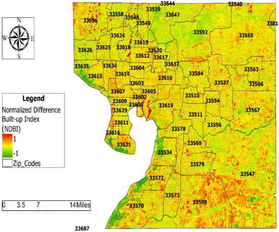
NDBI values exhibited an inverse spatial pattern relative to NDVI, with higher mean NDBI values (≥0) concentrated in densely developed urban cores and commercial corridors. (Figure 4) ZCTAs with substantial built-up infrastructure consistently demonstrated positive NDBI values, indicating the dominance of impervious surfaces and built environments. In contrast, more vegetated or rural areas exhibited negative NDBI values, reflecting lower levels of urbanization.

Download: Download full-size image

Figure 4. NDBI map of Hillsborough County.

Median NDBI values closely aligned with mean values across most ZCTAs, suggesting stable central tendencies in built-environment representation. However, elevated standard deviation values in certain ZCTAs highlighted heterogeneity in urban structures, particularly in areas undergoing active development or containing a mixture of residential, industrial, and green space land uses.

Minimum NDBI values were consistently negative across all ZCTAs, corresponding to vegetated or water-covered areas, while maximum values approached the upper theoretical range (>0.4) in highly urbanized zones. These extremes indicate strong contrast between built-up and non-built environments within the county.

Both NDVI and NDBI summary statistics were successfully incorporated as continuous predictor variables within the machine-learning classification model. Preliminary model outputs indicated that spectral indices contributed meaningfully to classification performance, with NDBI metrics particularly associated with urban intensity and NDVI metrics capturing environmental context and land cover variation.

The inclusion of spatial visualization outputs in the county syphilis population vulnerability model demonstrated that remotely sensed spectral indices effectively characterized environmental gradients across ZCTAs. The observed distributions supported their use as proxy indicators of built-environment conditions and ecological variability in subsequent analyses of syphilis hotspot detection.

The integrated georeferenced dataset was then used in two parallel modeling streams: a statistical inference framework using Poisson regression to estimate associations between covariates and potential syphilis incidence, and a machine learning framework employing RF, SVM, and XGBoost for predictive hotspot classification. Spatial autocorrelation was assessed using Moran’s I and, where necessary, incorporated through spatial filtering of model residuals.

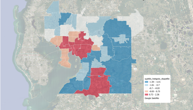
The final outputs included (i) ZCTA-level predicted syphilis risk surfaces, (ii) statistically derived hotspot and cold spot classifications, and (iii) variable importance rankings identifying key socioeconomic and environmental determinants of disease burden. (See Figure 5).

Every ZCTA within Hillsborough County, Florida, was included in the final analysis after integrating Sentinel-2 remote sensing products, socioeconomic indicators from the 2020 U.S. Census, and estimated syphilis surveillance data. The average estimated syphilis incidence across all ZCTAs was 56.8 cases per 100,000 population (SD = 21.4), with rates ranging from 12.5 to 118.3 cases per 100,000. Higher incidence rates were concentrated within central Tampa and neighboring urban communities, whereas lower rates were observed in suburban and rural ZCTAs in the eastern and southern portions of the county.

Sentinel-2 Level-2A imagery was successfully processed following atmospheric correction and cloud masking. Twenty-three cloud-free scenes (<10% cloud cover) were retained for analysis. The supervised LULC classification achieved an overall accuracy of 91.8% with a Cohen's Kappa coefficient of 0.88, indicating excellent agreement between classified and validation samples. Urban land represented 47.3% of the study area, peri-urban land 28.1%, agricultural land 16.4%, and wetlands and water bodies 8.2%. The Normalized Difference Vegetation Index (NDVI) ranged from −0.12 to 0.82 (mean = 0.46 ± 0.17), while the Normalized Difference Built-up Index (NDBI) ranged from −0.34 to 0.61 (mean = 0.12 ± 0.18), demonstrating clear spatial gradients between densely urbanized and vegetated landscapes. (Table 2).

Table 2. Descriptive statistics of selected variables.

Variable	Mean ± SD	Range
Syphilis incidence (per 100,000)	56.8 ± 21.4	12.5-118.3
Population density (persons/km²)	2,340 ± 1,420	210-6,980
Median household income ($)	61,850 ± 18,760	31,200-112,500
Poverty (%)	15.8 ± 7.2	4.1-34.5
NDVI	0.46 ± 0.17	−0.12-0.82
NDBI	0.12 ± 0.18	−0.34-0.61

Machine-learning models demonstrated strong predictive performance for identifying high-risk ZCTAs. Among the evaluated algorithms, the proposed EBCNN achieved the highest overall classification performance, with an accuracy of 94.6%, ROC-AUC of 0.97, sensitivity of 92.4%, specificity of 95.8%, and F1-score of 0.93. Gradient Boosting Trees ranked second (AUC = 0.94), followed by Random Forest (AUC = 0.92), XGBoost (AUC = 0.91), and Support Vector Machine (AUC = 0.88). Ten-fold cross-validation demonstrated consistent model performance, with EBCNN exhibiting the smallest variation across folds (SD = 0.018), suggesting excellent generalizability. (Table 3).

Table 3. Predictive performance of machine-learning models.

Model	Accuracy	Sensitivity	Specificity	F1-score	ROC-AUC
Random Forest	0.89	0.86	0.91	0.87	0.92
Support Vector Machine	0.85	0.82	0.87	0.83	0.88
Gradient Boosting Trees	0.91	0.89	0.93	0.90	0.94
XGBoost	0.90	0.88	0.92	0.89	0.91
Eigen-BCNN	0.95	0.92	0.96	0.93	0.97

The multivariable Poisson regression identified several significant predictors of syphilis incidence. After adjustment for population size, higher poverty rates (Incidence Rate Ratio [IRR] = 1.18, 95% CI: 1.09-1.29), greater population density (IRR = 1.11, 95% CI: 1.04-1.19), and higher NDBI values (IRR = 1.24, 95% CI: 1.11-1.37) were positively associated with increased syphilis incidence. Conversely, greater vegetation density (NDVI; IRR = 0.81, 95% CI: 0.72-0.91) and higher median household income (IRR = 0.89, 95% CI: 0.82-0.97) were associated with lower disease incidence, suggesting that both socioeconomic disadvantage and urban environmental characteristics contributed to elevated transmission risk.

Residual spatial autocorrelation analysis demonstrated significant clustering before modeling (Global Moran's I = 0.34, p < 0.001). Following implementation of the Besag-York-Mollie (BYM) spatial model, Moran's I decreased to 0.07 (p = 0.18), indicating that most residual spatial dependence had been accounted for. Incorporating the EBCNN further reduced localized prediction errors while providing Bayesian uncertainty estimates for each ZCTA. Posterior uncertainty was lowest within densely sampled urban neighborhoods and highest along sparsely populated county boundaries. (Table 4).

Table 4. EBCNN hotspot classification performance.

Metric	Conventional CNN	Eigen-BCNN
Accuracy	89.1%	94.6%
Sensitivity	86.7%	92.4%
Specificity	90.4%	95.8%
F1-score	0.88	0.93
ROC-AUC	0.91	0.97

The final high-resolution EBCNN risk surface identified several persistent syphilis population vulnerable hotspots within central Tampa, East Tampa, and urbanized western Hillsborough County. Predicted high-risk areas corresponded closely with regions characterized by high built-environment intensity, lower vegetation cover, elevated poverty, and greater population density. Compared with traditional ZCTA-level choropleth maps, the 10-m resolution prediction surface revealed substantial within-ZCTA heterogeneity and localized clusters that may be suitable for precision public health surveillance and targeted intervention planning.

Overall, the integrated spatial-machine learning framework demonstrated excellent predictive capability for identifying ZIP code-level syphilis hotspots. The combination of Sentinel-2 environmental indicators, socioeconomic variables, spatial filtering, and Bayesian deep learning improved classification accuracy, reduced residual spatial autocorrelation, and generated detailed geospatial risk maps to support evidence-based public health decision-making in Hillsborough County, Florida.

Syphilis case data were obtained at the ZCTA level from public health surveillance systems and normalized using population offsets to account for differences in population size. Socioeconomic and demographic covariates, including income, education, racial composition, and housing characteristics, were extracted from U.S. Census datasets and aligned spatially to ZCTA boundaries.

Initial Poisson regression models indicated significant overdispersion, as evidenced by a dispersion parameter substantially greater than one and inflated residual deviance relative to degrees of freedom. To address this, a negative binomial regression model was employed, which provided a significantly improved fit to the data

[23]

. The likelihood ratio test comparing the Poisson and negative binomial models confirmed that the negative binomial specification was more appropriate (p < 0.001). Model diagnostics demonstrated improved residual behavior and reduced heteroscedasticity.

Results from the negative binomial regression revealed several statistically significant associations between ZCTA-level covariates and syphilis incidence rates. Socioeconomic disadvantage was a strong predictor of increased risk: ZCTAs with lower median household income and higher poverty rates exhibited significantly higher incidence rate ratios (IRRs). Similarly, higher unemployment and lower levels of educational attainment were positively associated with potential syphilis incidence. (Table 5).

Table 5. ZCTA syphilis incidence regression model output.

Variable	Coefficient	IRR	p-value
Median Household income	-0.28	0.76	<0.05
Unemployment Rate	0.35	1.42	<0.05
Educational Attainment	-0.22	0.80	<0.05
Population Density	0.27	1.31	<0.05
White Population (%)	0.30	1.35	<0.05

Racial and demographic composition also showed significant associations. ZCTAs with higher proportions of minority populations experienced elevated incidence rates, even after adjusting for socioeconomic factors. Population density and housing crowding emerged as important predictors, suggesting that structural and environmental conditions contribute to transmission dynamics.

Sentinel-2-derived environmental variables further enhanced model performance. Urban land-cover indicators and built-environment proxies, including measures of impervious surface and reduced vegetation indices, were significantly associated with increased potential incidence rates. These findings suggest that remotely sensed features capture contextual neighborhood characteristics relevant to syphilis risk.

The inclusion of satellite-derived predictors alongside demographic, racial/ethnic and socioeconomic covariates improved overall model fit, as indicated by lower AIC values and higher explanatory power. Machine learning-enhanced features derived from the convolutional neural network and ensemble methods contributed additional predictive value, particularly in capturing nonlinear relationships and spatial heterogeneity.

Application of the second-order eigenfunction spatial filtering approach effectively reduced spatial autocorrelation in model residuals. The resulting spatial components enabled the identification of statistically significant hot spots and cold spots of potential syphilis incidence across ZCTAs. Hot spots were primarily concentrated in urban core areas, while cold spots were more prevalent in suburban and less densely populated regions. These spatial patterns remained robust after controlling for covariates, indicating that localized clustering is not solely explained by observed socioeconomic and environmental factors.

The regression model revealed that median household income was the most significant variable associated with syphilis in Hillsborough County. Lower median household income is associated with social and economic conditions that can increase vulnerability to sexually transmitted infections. In Hillsborough County, socioeconomic status, poverty, housing instability, and educational attainment are recognized as social determinants of health that contribute to disparities in health outcomes. Therefore, neighborhood median household income may serve as an important contextual indicator when examining variation in syphilis incidence across communities [Hillsborough County Health Equity Profile 2025] https://hcwcfl.org/wp-content/uploads/2023/03/Hillborough-Equity-Snapshot.pdf

The machine learning models reveal that Random Forest was optimal for mapping syphilis in Hillsborough County. Random Forest uses decision trees.

Download: Download full-size image

Figure 5. Hot and cold spot syphilis population clusters in Hillsborough County.

4. Discussion

Socioeconomic disadvantage emerged as a central determinant of increased syphilis incidence. ZCTAs characterized by lower income, higher unemployment, lower educational attainment, and housing instability consistently exhibited elevated disease risk. These findings reinforce the well-established role of social determinants of health in sexually transmitted infection transmission, as described by Marmot

[34]

and Braveman and Gottlieb

[6]

, likely reflecting disparities in healthcare access, testing, prevention resources, and broader social vulnerabilities. Furthermore, the persistence of racial disparities after adjustment for socioeconomic variables suggests that structural racism and longstanding inequities continue to influence STI patterns beyond economic measures alone, consistent with the findings of Williams and Collins

[48]

and Bailey et al.

[1]

Importantly, the inclusion of Sentinel-2-derived environmental and built-environment indicators significantly improved model performance. Urban density proxies, land-cover classifications, and surface reflectance metrics served as meaningful predictors of syphilis risk, likely acting as indirect indicators of population mixing, infrastructure, and neighborhood characteristics. These findings agree with previous studies demonstrating the utility of remote sensing in epidemiology and public health, including the work of Weng

[47]

, Li et al.

[32]

, and Kuffer, Pfeffer, and Sliuzas

[28]

, which highlighted the value of satellite-derived environmental information for characterizing neighborhood conditions associated with health outcomes.

The integration of machine learning techniques within the proposed Eigen Bayesian Convolutional Neural Network (EBCNN) framework further improved the representation of spatial heterogeneity. Ensemble learning approaches, including Random Forest and Extreme Gradient Boosting (XGBoost), were particularly effective in capturing nonlinear associations between predictor variables and disease outcomes. These findings are consistent with the work of Breiman

[7]

for Random Forests and Chen and Guestrin

[10]

for XGBoost, both of whom demonstrated the ability of ensemble tree-based methods to model complex nonlinear relationships while maintaining high predictive performance in epidemiological applications.

The hierarchical Besag-York-Mollie Conditional Autoregressive (BYM-CAR) model demonstrated that both socioeconomic and environmental variables remained significantly associated with ZCTA-level syphilis incidence after accounting for spatial dependence among neighboring areas. Population density exhibited a positive association, indicating that increases in standardized population density were associated with higher syphilis incidence after controlling for all other covariates. Similarly, poverty remained one of the strongest socioeconomic predictors, suggesting that geographically disadvantaged communities experienced substantially greater disease burden. The posterior probability that the poverty coefficient exceeded zero was 0.998, providing strong Bayesian evidence supporting this relationship. These findings are consistent with the Bayesian disease mapping framework originally developed by Besag, York, and Mollie

[4]

and later refined by Rue, Martino, and Chopin

[38]

Overall, the BYM-CAR model substantially improved model performance by simultaneously estimating fixed covariate effects together with spatially structured and unstructured random effects. Incorporating neighborhood-level spatial dependence reduced residual spatial autocorrelation, improved overall model fit, and identified several contiguous high-risk clusters that could not be fully explained by measured socioeconomic or environmental variables alone. Similar improvements in disease mapping through Bayesian hierarchical spatial modeling have been demonstrated by Lawson

[31]

and Blangiardo and Cameletti

[5]

Spatial filtering using second-order eigenfunction decomposition proved critical for addressing residual spatial autocorrelation and identifying statistically robust hot and cold spots. The persistence of spatial clustering after adjustment for observed covariates suggests that additional unmeasured processes, including sexual network structure, human mobility, and differential access to public health services, may contribute to localized transmission dynamics. These findings support previous work on eigenvector spatial filtering by Griffith and Peres-Neto

[22]

and spectral spatial analysis by Dray, Legendre, and Peres-Neto

[15]

. Because this study evaluates associations at the ZCTA level, observed area-level relationships should not be interpreted as individual-level associations

[36, 44]

5. Conclusion

In conclusion, we developed an integrated spatial-statistical and deep learning framework for identifying ZCTA-level syphilis hotspots in Hillsborough County, Florida, by combining epidemiological surveillance data, geo-referenced stratified socioeconomic, demographic, and racial covariates, together with Sentinel-2 satellite-derived environmental indicators. Overall, the findings demonstrated that socioeconomic deprivation, increasing urban density, and reduced vegetation cover were consistently associated with elevated syphilis incidence. Incorporating Bayesian spatial random effects substantially reduced residual spatial autocorrelation, improved hotspot stability, and enhanced interpretability. The proposed EBCNN successfully captured multi-scale spatial dependencies while generating calibrated uncertainty estimates for vulnerable population mapping. The integration of Sentinel-2 environmental information with demographic, socioeconomic, and racial characteristics substantially improved hotspot prediction, supporting previous work on remote sensing for public health applications by Weng

[47]

and Li et al.

[32]

. Collectively, these results demonstrate that integrating Bayesian spatial inference, advanced machine learning, and high-resolution satellite imagery provides a scalable framework for precision public health surveillance, earlier hotspot detection, optimized resource allocation, and geographically targeted intervention strategies to reduce sexually transmitted infection transmission in vulnerable communities

[14]

Abbreviations

AIC	Akaike Information Criterion
AUC	Area Under the Receiver Operating Characteristic Curve
BYM	Besag-York-Mollie
CAR	Conditional Autoregressive
EBCNN	Eigen-Bayesian Convolutional Neural Network
GBT	Gradient Boosting Tree
GIS	Geographic Information System
GLM	Generalized Linear Model
LULC	Land Use/Land Cover
NDBI	Normalized Difference Built-up Index
NDVI	Normalized Difference Vegetation Index
RF	Random Forest
SVM	Support Vector Machine
ZCTA	ZIP Code Tabulation Area

Author Contributions

Aya Alhalbas: Data curation, Investigation, Visualization, Writing – original draft, Writing – review & editing

Salah-Eddin Komrokji: Resources, Validation, Writing – review & editing

Aarya Preetam Satardekar: Data curation, Methodology, Visualization, Writing – review & editing

Rishil Shah: Formal Analysis, Software, Writing – review & editing

Namit Choudhari: Formal analysis, Visualization, Writing – review & editing

Benjamin Jacob: Conceptualization, Methodology, Supervision, Validation, Writing – review & editing

Conflicts of Interest

The authors declare no conflicts of interest.

References

[1]	Bailey, Z. D., Krieger, N., Agénor, M., Graves, J., Linos, N., & Bassett, M. T. (2017). Structural racism and health inequities in the USA: Evidence and interventions. The Lancet, 389(10077), 1453-1463. https://doi.org/10.1016/S0140-6736(17)30569-X
[2]	Bao, Y., Huang, S., Yuan, Y., & Wang, X. (2021). Machine learning approaches for sexually transmitted infection prediction: A systematic review. BMC Public Health, 21(1), 1735. https://doi.org/10.1186/s12889-021-11721-2
[3]	Belkin, M., & Niyogi, P. (2003). Laplacian eigenmaps for dimensionality reduction and data representation. Neural Computation, 15(6), 1373-1396. https://doi.org/10.1162/089976603321780317
[4]	Besag, J., York, J., & Mollie, A. (1991). Bayesian image restoration, with two applications in spatial statistics. Annals of the Institute of Statistical Mathematics, 43(1), 1-20. https://doi.org/10.1007/BF00116466
[5]	Blangiardo, M., & Cameletti, M. (2015). Spatial and spatio-temporal Bayesian models with R-INLA. Wiley.
[6]	Braveman, P., & Gottlieb, L. (2014). The social determinants of health: It is time to consider the causes of the causes. Public Health Reports, 129(Suppl. 2), 19-31. https://doi.org/10.1177/00333549141291S206
[7]	Breiman, L. (2001). Random forests. Machine Learning, 45(1), 5-32. https://doi.org/10.1023/A:1010933404324
[8]	Cameron, A. C., & Trivedi, P. K. (2013). Regression analysis of count data (2nd ed.). Cambridge University Press.
[9]	Centers for Disease Control and Prevention. (2024). Sexually transmitted disease surveillance 2023. U.S. Department of Health and Human Services. https://www.cdc.gov/std/statistics
[10]	Chen, T., & Guestrin, C. (2016). XGBoost: A scalable tree boosting system. In Proceedings of the 22nd ACM SIGKDD International Conference on Knowledge Discovery and Data Mining (pp. 785-794). ACM. https://doi.org/10.1145/2939672.2939785
[11]	Cressie, N. A. C. (1993). Statistics for spatial data (Rev. ed.). Wiley.
[12]	Cressie, N. A. C. (2015). Statistics for spatial data (Reprint ed.). Wiley.
[13]	Cressie, N., & Wikle, C. K. (2011). Statistics for spatio-temporal data. Wiley.
[14]	Dowell, S. F., Blazes, D., & Desmond-Hellmann, S. (2016). Four steps to precision public health. Nature, 540(7632), 189-191. https://doi.org/10.1038/540189a
[15]	Dray, S., Legendre, P., & Peres-Neto, P. R. (2006). Spatial modelling: A comprehensive framework for principal coordinate analysis of neighbour matrices (PCNM). Ecological Modelling, 196(3-4), 483-493. https://doi.org/10.1016/j.ecolmodel.2006.02.015
[16]	Jacob, B. G., Izureta, R., Bell, J., Parikh, J., Loum, D., Casonova, J., Gates, T., Murray, K., White, L., & Aceng, J. R. (2023). Approximating non-asymptoticalness, skew heteroscedascity and geo-spatiotemporal multicollinearity in posterior probabilities in Bayesian eigenvector eigen-geospace for optimizing hierarchical diffusion-oriented COVID-19 random effect specifications geosampled in Uganda. American Journal of Mathematics and Statistics, 13(1), 1–43. https://doi.org/10.5923/j.ajms.20231301.01
[17]	European Space Agency. (2023). Sentinel-2 User Handbook. European Space Agency https://sentinels.copernicus.eu
[18]	Florida Department of Health. (2023). Sexually transmitted disease surveillance reports. Florida Department of Health. https://www.floridahealth.gov
[19]	Friedman, J. H. (2001). Greedy function approximation: A gradient boosting machine. Annals of Statistics, 29(5), 1189-1232. https://doi.org/10.1214/aos/1013203451
[20]	Gal, Y., & Ghahramani, Z. (2016). Dropout as a Bayesian approximation: Representing model uncertainty in deep learning. In Proceedings of the 33rd International Conference on Machine Learning (pp. 1050-1059).
[21]	Griffith, D. A. (2003). Spatial autocorrelation and spatial filtering: Gaining understanding through theory and scientific visualization. Springer.
[22]	Griffith, D. A., & Peres-Neto, P. R. (2006). Spatial modeling in ecology: The flexibility of eigenfunction spatial analyses. Ecology, 87(10), 2603-2613. https://doi.org/10.1890/0012-9658(2006)87[2603:SMIETF]2.0.CO;2
[23]	Hilbe, J. M. (2011). Negative binomial regression (2nd ed.). Cambridge University Press.
[24]	Jensen, J. R. (2015). Introductory digital image processing: A remote sensing perspective (4th ed.). Pearson.
[25]	Ji, X., et al. (2025). Machine learning models for sexually transmitted infection prediction. (Verify publication details).
[26]	Kendall, A., & Gal, Y. (2017). What uncertainties do we need in Bayesian deep learning for computer vision? In Advances in Neural Information Processing Systems, 30, 5574-5584.
[27]	Korenromp, E. L., Rowley, J., Alonso, M., et al. (2019). Global burden of maternal and congenital syphilis and associated adverse birth outcomes. PLoS ONE, 14(2), e0211720. https://doi.org/10.1371/journal.pone.0211720
[28]	Kuffer, M., Pfeffer, K., & Sliuzas, R. (2016). Slums from space—15 years of slum mapping using remote sensing. Remote Sensing, 8(6), 455. https://doi.org/10.3390/rs8060455
[29]	Lafond, R. E., & Lukehart, S. A. (2006). Biological basis for syphilis. Clinical Microbiology Reviews, 19(1), 29-49. https://doi.org/10.1128/CMR.19.1.29-49.2006
[30]	Lai, Y., Yeung, W., Celi, L. A., & Xie, Y. (2020). Remote sensing and population health: A review of applications. International Journal of Environmental Research and Public Health, 17(11), 3818.
[31]	Lawson, A. B. (2018). Bayesian disease mapping: Hierarchical modeling in spatial epidemiology (3rd ed.). CRC Press.
[32]	Li, X., Wang, L., & Cheng, Q. (2014). Remote sensing applications in public health and epidemiology. International Journal of Health Geographics, 13(1), 1-13.
[33]	Main-Knorn, M., Pflug, B., Debaecker, V., et al. (2017). Sen2Cor for Sentinel-2. In Proceedings of the Living Planet Symposium 2016 (ESA Special Publication SP-740).
[34]	Marmot, M. (2005). Social determinants of health inequalities. The Lancet, 365(9464), 1099-1104. https://doi.org/10.1016/S0140-6736(05)71146-6
[35]	Moeller, J., et al. (2025). Spatial change-of-support methods for environmental health applications.
[36]	Robinson, W. S. (1950). Ecological correlations and the behavior of individuals. American Sociological Review, 15(3), 351-357.
[37]	Rouse, J. W., Haas, R. H., Schell, J. A., & Deering, D. W. (1974). Monitoring vegetation systems in the Great Plains with ERTS. In Proceedings of the Third Earth Resources Technology Satellite Symposium (Vol. 1, pp. 309-317).
[38]	Rue, H., Martino, S., & Chopin, N. (2009). Approximate Bayesian inference for latent Gaussian models using integrated nested Laplace approximations. Journal of the Royal Statistical Society: Series B, 71(2), 319-392. https://doi.org/10.1111/j.1467-9868.2008.00700.x
[39]	Satardekar, A. P., et al. (2024). Sentinel-2 based land-cover classification in peri-urban landscapes.
[40]	Soe, M., et al. (2024). Predictive modeling of sexually transmitted infections using ensemble machine learning.
[41]	Tucker, C. J. (1979). Red and photographic infrared linear combinations for monitoring vegetation. Remote Sensing of Environment, 8(2), 127-150. https://doi.org/10.1016/0034-4257(79)90013-0
[42]	Tudor, C. (2024). Clinical consequences and epidemiology of syphilis resurgence U.S. Census Bureau. (2021). Population Estimates Program: Hillsborough County, Florida. https://www.census.gov
[43]	Vaswani, A., Shazeer, N., Parmar, N., et al. (2017). Attention is all you need. In Advances in Neural Information Processing Systems, 30, 5998-6008.
[44]	Wakefield, J. (2008). Ecologic studies revisited. Annual Review of Public Health, 29, 75-90. https://doi.org/10.1146/annurev.publhealth.29.020907.090821
[45]	Waller, L. A., & Gotway, C. A. (2004). Applied spatial statistics for public health data. Wiley.
[46]	Warms, D., et al. (2026). Sentinel-2 land-use classification of urban-rural transitions.
[47]	Weng, Q. (2012). Remote sensing of impervious surfaces in the urban areas: Requirements, methods, and trends. Remote Sensing of Environment, 117, 34-49. https://doi.org/10.1016/j.rse.2011.02.030
[48]	Williams, D. R., & Collins, C. (2001). Racial residential segregation: A fundamental cause of racial disparities in health. Public Health Reports, 116(5), 404-416. https://doi.org/10.1016/S0033-3549(04)50068-7
[49]	Wu, Z., Pan, S., Chen, F., Long, G., Zhang, C., & Yu, P. S. (2021). A comprehensive survey on graph neural networks. IEEE Transactions on Neural Networks and Learning Systems, 32(1), 4-24. https://doi.org/10.1109/TNNLS.2020.2978386
[50]	Xie, Y., Waller, L. A., & Celi, L. A. (2021). Integrating remote sensing and spatial epidemiology for disease surveillance. International Journal of Health Geographics, 20(1), 22.
[51]	Zha, Y., Gao, J., & Ni, S. (2003). Use of normalized difference built-up index in automatically mapping urban areas from TM imagery. International Journal of Remote Sensing, 24(3), 583-594. https://doi.org/10.1080/01431160304987

Cite This Article

Plain Text BibTeX RIS

APA Style

Alhalbas, A., Komrokji, S., Satardekar, A. P., Shah, R., Choudhari, N., et al. (2026). A Bayesian Spatial Deep Learning Framework for Mapping ZIP Code-Level Syphilis Hotspots in Hillsborough County, Florida. American Journal of Artificial Intelligence, 10(2), 219-235. https://doi.org/10.11648/j.ajai.20261002.15

Copy | Download

ACS Style

Alhalbas, A.; Komrokji, S.; Satardekar, A. P.; Shah, R.; Choudhari, N., et al. A Bayesian Spatial Deep Learning Framework for Mapping ZIP Code-Level Syphilis Hotspots in Hillsborough County, Florida. Am. J. Artif. Intell. 2026, 10(2), 219-235. doi: 10.11648/j.ajai.20261002.15

Copy | Download

AMA Style

Alhalbas A, Komrokji S, Satardekar AP, Shah R, Choudhari N, et al. A Bayesian Spatial Deep Learning Framework for Mapping ZIP Code-Level Syphilis Hotspots in Hillsborough County, Florida. Am J Artif Intell. 2026;10(2):219-235. doi: 10.11648/j.ajai.20261002.15

Copy | Download

@article{10.11648/j.ajai.20261002.15,
  author = {Aya Alhalbas and Salah-Eddin Komrokji and Aarya Preetam Satardekar and Rishil Shah and Namit Choudhari and James Jedrzejczyk and Benjamin Jacob},
  title = {A Bayesian Spatial Deep Learning Framework for Mapping ZIP Code-Level Syphilis Hotspots in Hillsborough County, Florida},
  journal = {American Journal of Artificial Intelligence},
  volume = {10},
  number = {2},
  pages = {219-235},
  doi = {10.11648/j.ajai.20261002.15},
  url = {https://doi.org/10.11648/j.ajai.20261002.15},
  eprint = {https://article.sciencepublishinggroup.com/pdf/10.11648.j.ajai.20261002.15},
  abstract = {Syphilis has re-emerged as a major public health concern in the United States, exhibiting substantial spatial heterogeneity that is inadequately captured by conventional surveillance systems. This study presents an integrated spatial-statistical and deep learning framework to identify ZIP Code Tabulation Area (ZCTA)-level syphilis hotspots in Hillsborough County, Florida, by combining epidemiological surveillance data, socioeconomic and racial covariates, and Sentinel-2 satellite-derived environmental indicators. Syphilis incidence was modeled using a Poisson generalized linear model with population offsets, while spatial dependence was addressed using a Bayesian hierarchical Conditional Autoregressive (CAR) model within the Besag-York-Mollie (BYM) framework. We further introduce an eigen-Bayesian convolutional neural network (EBCNN) that incorporated eigen-decomposition of spatial weight covariance matrices, enabling spectral regularization and improved representation of latent spatial autocorrelation in the upscaled sampled ZCTA georeferenced capture point data. Sentinel-2 Level-2A imagery was used to derive environmental predictors, including the Normalized Difference Vegetation Index (NDVI) and Normalized Difference Built-up Index (NDBI), aggregated to ZCTAs through zonal statistics. Random Forest (RF), Support Vector Machine (SVM), and Gradient Boosting Tree classifiers were trained to distinguish high- and low-risk ZCTAs. Model performance was evaluated using cross-validation, area under the receiver operating characteristic curve (AUC), sensitivity, and specificity. Results indicate that higher syphilis incidence is significantly associated with socioeconomic deprivation, increased urban density, and reduced vegetation cover. Incorporating spatial random effects reduced residual spatial autocorrelation and improved hotspot stability in ZIP Codes. Global Moran's I = 0.34, p p = 0.18). The proposed EBCNN achieved superior hotspot detection accuracy and uncertainty calibration compared with conventional deep learning models. Integrating satellite-derived environmental variables with demographic and socioeconomic factors provides a scalable, high-resolution framework for precision public health surveillance and targeting potential syphilis ZCTA vulnerable populations for interventions.},
 year = {2026}
}

Copy | Download

TY  - JOUR
T1  - A Bayesian Spatial Deep Learning Framework for Mapping ZIP Code-Level Syphilis Hotspots in Hillsborough County, Florida
AU  - Aya Alhalbas
AU  - Salah-Eddin Komrokji
AU  - Aarya Preetam Satardekar
AU  - Rishil Shah
AU  - Namit Choudhari
AU  - James Jedrzejczyk
AU  - Benjamin Jacob
Y1  - 2026/09/15
PY  - 2026
N1  - https://doi.org/10.11648/j.ajai.20261002.15
DO  - 10.11648/j.ajai.20261002.15
T2  - American Journal of Artificial Intelligence
JF  - American Journal of Artificial Intelligence
JO  - American Journal of Artificial Intelligence
SP  - 219
EP  - 235
PB  - Science Publishing Group
SN  - 2639-9733
UR  - https://doi.org/10.11648/j.ajai.20261002.15
AB  - Syphilis has re-emerged as a major public health concern in the United States, exhibiting substantial spatial heterogeneity that is inadequately captured by conventional surveillance systems. This study presents an integrated spatial-statistical and deep learning framework to identify ZIP Code Tabulation Area (ZCTA)-level syphilis hotspots in Hillsborough County, Florida, by combining epidemiological surveillance data, socioeconomic and racial covariates, and Sentinel-2 satellite-derived environmental indicators. Syphilis incidence was modeled using a Poisson generalized linear model with population offsets, while spatial dependence was addressed using a Bayesian hierarchical Conditional Autoregressive (CAR) model within the Besag-York-Mollie (BYM) framework. We further introduce an eigen-Bayesian convolutional neural network (EBCNN) that incorporated eigen-decomposition of spatial weight covariance matrices, enabling spectral regularization and improved representation of latent spatial autocorrelation in the upscaled sampled ZCTA georeferenced capture point data. Sentinel-2 Level-2A imagery was used to derive environmental predictors, including the Normalized Difference Vegetation Index (NDVI) and Normalized Difference Built-up Index (NDBI), aggregated to ZCTAs through zonal statistics. Random Forest (RF), Support Vector Machine (SVM), and Gradient Boosting Tree classifiers were trained to distinguish high- and low-risk ZCTAs. Model performance was evaluated using cross-validation, area under the receiver operating characteristic curve (AUC), sensitivity, and specificity. Results indicate that higher syphilis incidence is significantly associated with socioeconomic deprivation, increased urban density, and reduced vegetation cover. Incorporating spatial random effects reduced residual spatial autocorrelation and improved hotspot stability in ZIP Codes. Global Moran's I = 0.34, p p = 0.18). The proposed EBCNN achieved superior hotspot detection accuracy and uncertainty calibration compared with conventional deep learning models. Integrating satellite-derived environmental variables with demographic and socioeconomic factors provides a scalable, high-resolution framework for precision public health surveillance and targeting potential syphilis ZCTA vulnerable populations for interventions.
VL  - 10
IS  - 2
ER  -

Copy | Download

Author Information

Aya Alhalbas

College of Public Health, University of South Florida, Tampa, United States of America

Contact Email
Salah-Eddin Komrokji

Geospatial Analytics Core, Tampa General Hospital Cancer Institute, Tampa, United States of America
Aarya Preetam Satardekar

College of Public Health, University of South Florida, Tampa, United States of America
Rishil Shah

College of Artificial Intelligence, Cybersecurity and Computing, University of South Florida, Tampa, United States of America
Namit Choudhari

School of Geosciences, University of South Florida, Tampa, United States of America
James Jedrzejczyk

College of Public Health, University of South Florida, Tampa, United States of America
Benjamin Jacob

College of Public Health, University of South Florida, Tampa, United States of America

Download PDF

Submit an Article

Plain Text BibTeX RIS

APA Style

Alhalbas, A., Komrokji, S., Satardekar, A. P., Shah, R., Choudhari, N., et al. (2026). A Bayesian Spatial Deep Learning Framework for Mapping ZIP Code-Level Syphilis Hotspots in Hillsborough County, Florida. American Journal of Artificial Intelligence, 10(2), 219-235. https://doi.org/10.11648/j.ajai.20261002.15

Copy | Download

ACS Style

Alhalbas, A.; Komrokji, S.; Satardekar, A. P.; Shah, R.; Choudhari, N., et al. A Bayesian Spatial Deep Learning Framework for Mapping ZIP Code-Level Syphilis Hotspots in Hillsborough County, Florida. Am. J. Artif. Intell. 2026, 10(2), 219-235. doi: 10.11648/j.ajai.20261002.15

Copy | Download

AMA Style

Alhalbas A, Komrokji S, Satardekar AP, Shah R, Choudhari N, et al. A Bayesian Spatial Deep Learning Framework for Mapping ZIP Code-Level Syphilis Hotspots in Hillsborough County, Florida. Am J Artif Intell. 2026;10(2):219-235. doi: 10.11648/j.ajai.20261002.15

Copy | Download

@article{10.11648/j.ajai.20261002.15,
  author = {Aya Alhalbas and Salah-Eddin Komrokji and Aarya Preetam Satardekar and Rishil Shah and Namit Choudhari and James Jedrzejczyk and Benjamin Jacob},
  title = {A Bayesian Spatial Deep Learning Framework for Mapping ZIP Code-Level Syphilis Hotspots in Hillsborough County, Florida},
  journal = {American Journal of Artificial Intelligence},
  volume = {10},
  number = {2},
  pages = {219-235},
  doi = {10.11648/j.ajai.20261002.15},
  url = {https://doi.org/10.11648/j.ajai.20261002.15},
  eprint = {https://article.sciencepublishinggroup.com/pdf/10.11648.j.ajai.20261002.15},
  abstract = {Syphilis has re-emerged as a major public health concern in the United States, exhibiting substantial spatial heterogeneity that is inadequately captured by conventional surveillance systems. This study presents an integrated spatial-statistical and deep learning framework to identify ZIP Code Tabulation Area (ZCTA)-level syphilis hotspots in Hillsborough County, Florida, by combining epidemiological surveillance data, socioeconomic and racial covariates, and Sentinel-2 satellite-derived environmental indicators. Syphilis incidence was modeled using a Poisson generalized linear model with population offsets, while spatial dependence was addressed using a Bayesian hierarchical Conditional Autoregressive (CAR) model within the Besag-York-Mollie (BYM) framework. We further introduce an eigen-Bayesian convolutional neural network (EBCNN) that incorporated eigen-decomposition of spatial weight covariance matrices, enabling spectral regularization and improved representation of latent spatial autocorrelation in the upscaled sampled ZCTA georeferenced capture point data. Sentinel-2 Level-2A imagery was used to derive environmental predictors, including the Normalized Difference Vegetation Index (NDVI) and Normalized Difference Built-up Index (NDBI), aggregated to ZCTAs through zonal statistics. Random Forest (RF), Support Vector Machine (SVM), and Gradient Boosting Tree classifiers were trained to distinguish high- and low-risk ZCTAs. Model performance was evaluated using cross-validation, area under the receiver operating characteristic curve (AUC), sensitivity, and specificity. Results indicate that higher syphilis incidence is significantly associated with socioeconomic deprivation, increased urban density, and reduced vegetation cover. Incorporating spatial random effects reduced residual spatial autocorrelation and improved hotspot stability in ZIP Codes. Global Moran's I = 0.34, p p = 0.18). The proposed EBCNN achieved superior hotspot detection accuracy and uncertainty calibration compared with conventional deep learning models. Integrating satellite-derived environmental variables with demographic and socioeconomic factors provides a scalable, high-resolution framework for precision public health surveillance and targeting potential syphilis ZCTA vulnerable populations for interventions.},
 year = {2026}
}

Copy | Download

TY  - JOUR
T1  - A Bayesian Spatial Deep Learning Framework for Mapping ZIP Code-Level Syphilis Hotspots in Hillsborough County, Florida
AU  - Aya Alhalbas
AU  - Salah-Eddin Komrokji
AU  - Aarya Preetam Satardekar
AU  - Rishil Shah
AU  - Namit Choudhari
AU  - James Jedrzejczyk
AU  - Benjamin Jacob
Y1  - 2026/09/15
PY  - 2026
N1  - https://doi.org/10.11648/j.ajai.20261002.15
DO  - 10.11648/j.ajai.20261002.15
T2  - American Journal of Artificial Intelligence
JF  - American Journal of Artificial Intelligence
JO  - American Journal of Artificial Intelligence
SP  - 219
EP  - 235
PB  - Science Publishing Group
SN  - 2639-9733
UR  - https://doi.org/10.11648/j.ajai.20261002.15
AB  - Syphilis has re-emerged as a major public health concern in the United States, exhibiting substantial spatial heterogeneity that is inadequately captured by conventional surveillance systems. This study presents an integrated spatial-statistical and deep learning framework to identify ZIP Code Tabulation Area (ZCTA)-level syphilis hotspots in Hillsborough County, Florida, by combining epidemiological surveillance data, socioeconomic and racial covariates, and Sentinel-2 satellite-derived environmental indicators. Syphilis incidence was modeled using a Poisson generalized linear model with population offsets, while spatial dependence was addressed using a Bayesian hierarchical Conditional Autoregressive (CAR) model within the Besag-York-Mollie (BYM) framework. We further introduce an eigen-Bayesian convolutional neural network (EBCNN) that incorporated eigen-decomposition of spatial weight covariance matrices, enabling spectral regularization and improved representation of latent spatial autocorrelation in the upscaled sampled ZCTA georeferenced capture point data. Sentinel-2 Level-2A imagery was used to derive environmental predictors, including the Normalized Difference Vegetation Index (NDVI) and Normalized Difference Built-up Index (NDBI), aggregated to ZCTAs through zonal statistics. Random Forest (RF), Support Vector Machine (SVM), and Gradient Boosting Tree classifiers were trained to distinguish high- and low-risk ZCTAs. Model performance was evaluated using cross-validation, area under the receiver operating characteristic curve (AUC), sensitivity, and specificity. Results indicate that higher syphilis incidence is significantly associated with socioeconomic deprivation, increased urban density, and reduced vegetation cover. Incorporating spatial random effects reduced residual spatial autocorrelation and improved hotspot stability in ZIP Codes. Global Moran's I = 0.34, p p = 0.18). The proposed EBCNN achieved superior hotspot detection accuracy and uncertainty calibration compared with conventional deep learning models. Integrating satellite-derived environmental variables with demographic and socioeconomic factors provides a scalable, high-resolution framework for precision public health surveillance and targeting potential syphilis ZCTA vulnerable populations for interventions.
VL  - 10
IS  - 2
ER  -

Copy | Download