A Comparative Study of Machine Learning-Based Predictive Models for House Price Prediction

Praveen Kumar Singh; Rachna Jain; Shikha Sharma

doi:doi:10.11648/j.sjbm.20261403.15

Research Article |

| Peer-Reviewed

A Comparative Study of Machine Learning-Based Predictive Models for House Price Prediction

Praveen Kumar Singh

, Rachna Jain^*

, Shikha Sharma

Published in Science Journal of Business and Management (Volume 14, Issue 3)

Received: 16 February 2026 Accepted: 15 June 2026 Published: 8 September 2026

Views: Downloads:

Download PDF

Share This Article

Twitter
Linked In
Facebook

Abstract

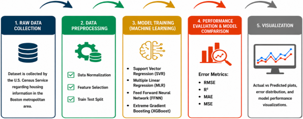
Predicting house prices is vital in helping homebuyers, investors, real estate agencies, and policymakers make informed decisions. But it's hard to precisely value a house when there are a number of factors at play – from property details to location to market conditions. The present study accounts for the comparative analysis of four machine learning techniques Multiple Linear Regression (MLR), Support Vector Regression (SVR), Feed Forward Neural Network (FFNN) and Extreme Gradient Boosting (XGBoost)) on predicting house prices by applying the Boston Housing dataset. Root Mean Square Error (RMSE), Mean Absolute Error (MAE), Mean Squared Error (MSE), and Coefficient of Determination (R²) were used to assess the models. Experimental results showed that XGBoost had the lowest RMSE (3.9147), MAE (2.8454), MSE (15.3252) and the highest R² value (0.7910) among all the models. The second best result was obtained by SVR while FFNN gave an accurate prediction and MLR gave the least accurate result. The analysis results show that the XGBoost model can better capture the complex nonlinear relationship between house attributes and makes it significantly better than the traditional regression model and neural network model. In conclusion, XGBoost is a powerful and stable model that can be used to accurately predict house prices and value real estate.

Published in	Science Journal of Business and Management (Volume 14, Issue 3) This article belongs to the Special Issue Global Challenges in Business: Rethinking Innovations and Sustainability
DOI	10.11648/j.sjbm.20261403.15
Page(s)	89-97
Creative Commons	This is an Open Access article, distributed under the terms of the Creative Commons Attribution 4.0 International License (http://creativecommons.org/licenses/by/4.0/), which permits unrestricted use, distribution and reproduction in any medium or format, provided the original work is properly cited.
Copyright	Copyright © The Author(s), 2026. Published by Science Publishing Group

Keywords

Machine Learning, Multiple Linear Regression, Feed-forward Neural Network, XGBoost, Support Vector Regression, House Price

1. Introduction

Housing has been identified as one of the key indicators of economic development and social wellbeing of any Nation. Greater economic growth generally leads to greater urbanization as people move to metropolitan regions to find better opportunities and a better life

[1]

. This population shift leads to increased demand for residential property and, in turn, affects residential property prices. Local infrastructure improvements, such as transportation systems, electricity, water supply, and public service facilities, can also significantly boost property value, besides the demand-driven factors. Thus, when the residential areas undergo infrastructure development, their housing price appreciation is noticeable

[2]

Today's society is a product of the advancement of science and technology, which has made everything more efficient, easily accessible, and improved. The use of Information and Communication Technology (ICT) is a part of many sectors and is continuously bringing out new solutions to help the economic and social development. While some technological advances have come with their own set of problems, most have had a positive influence, allowing for better decision-making and automation in many areas

[3]

One of these innovations is Artificial Intelligence (AI) and Machine Learning (ML), which have proven to be a significant asset for data analysis and forecasting. Machine learning is the name given to the field of AI that allows computer systems to learn how to recognize patterns and relationships from past data without needing to be explicitly programmed to do so. Machine learning techniques can be used for classification, clustering, association analysis, and regression problems, depending on the problem at hand. These techniques can help create predictive models that can forecast future results and analytical models that can extract meaningful information from large amounts of data

[4]

In contrast to traditional programming, machine learning algorithms learn the relationships between the inputs and outputs without any prior knowledge of how to program them, based on past observations. Machine learning approaches are broadly classified into three types: supervised learning, unsupervised learning, and reinforcement learning, depending on their learning approaches. For supervised learning, algorithms are trained on labelled data sets to find a mapping between input features and output. In this study, a number of supervised machine learning algorithms are used for the Boston Housing dataset to build predictive models for predicting house prices. The selected algorithms are trained from past attributes of houses, and then tested using suitable performance metrics. By comparing these models, one can gain insights into their effectiveness and suitability for housing price prediction applications

[5]

2. Literature Review

There have been many studies focusing on house price prediction using different datasets, methods, and machine learning techniques and with different prediction accuracy. Overall, there are several factors that affect house prices. Malang et al.

[6]

divided these factors into location, concept and physical characteristics. Physical characteristics are: property size, number of rooms, size of kitchen, size of garage, access to outside areas, land and building area and property age. Likewise, Kang et al. reported that factors like floor area, construction year, number of bedrooms and bathrooms, and interior facilities are significant factors affecting housing prices

[7]

. Conceptual aspect: marketing development strategies to entice prospective purchasers and investors. Moreover, high levels of access to key amenities like highways, airports, shopping centers, hospitals, and educational institutions will make a huge difference when it comes to property values. Some of these factors, including location, have a direct impact on land value and market demand. For home buyers, it is important to understand the trends in housing prices and the factors that contribute to them, but it is also crucial for homeowners, real estate operators, policy makers and city planners. The right prediction systems can help in making appropriate decisions in the purchase and investment of a home

[9-12]

. Middle income households also have a large stake in residential real estate, and it also provides them with collateral for entrepreneurial and investment activities. Housing prices, however, can have a positive effect on consumption because of rapid increases in housing values, but at the same time can have negative implications for financial stability due to the increased level of household debt. Various modeling techniques have been proposed to forecast house prices... Sean et al. analyzed how common economic shocks, disposable income, borrowing costs, demographic growth and spatial factors affected house prices at a state-level in the United States

[13]

. Using the Boston Housing dataset, Mu et al. applied machine learning algorithms to analyze the dataset, including Support Vector Machine (SVM), Least Squares Support Vector Machine (LSSVM), and Partial Least Squares (PLS)

[14]

. Similarly, Bahia et al. studied house price forecasting in the real estate sector with the use of data mining techniques, and created neural network models, namely Feedforward Neural Networks (FFNN) and Cascade Forward Neural Networks (CFNN) that increased the accuracy of predictions

[15]

. Multiple Linear Regression (MLR) and Extreme Gradient Boosting (XGBoost) are widely employed techniques for house price prediction. MLR is valued for its simplicity, interpretability, and ability to model relationships between housing prices and explanatory variables, making it a common baseline model

[19, 20]

. In contrast, XGBoost effectively captures complex nonlinear interactions among housing attributes through its gradient boosting framework. Several studies have demonstrated that XGBoost achieves higher prediction accuracy and better generalization performance than traditional regression models. Consequently, both approaches are extensively used in real estate valuation, with XGBoost often emerging as the superior predictive model

[17, 18]

3. Methodology

The general methodology used in the prediction of house prices is presented in Figure 1. The methodology is divided into five major steps: data collection, data pre-processing, model development, performance evaluation, and visualization of results. All stages are intended to ensure the forecasting models developed at each stage have high prediction accuracy. Firstly, the data collection after this preprocessing of the input dataset in a comprehensive manner to enhance the quality of the data and to make it suitable for machine learning applications. Following this, the preprocessed data is further used for the training of the models, which are developed as Support Vector Regression (SVR), Multiple Linear Regression (MLR), Feed Forward Neural Network (FNN), and Extreme Gradient Boosting (XGBoost) and then compared. The model development is followed by several statistical performance measures, such as Root Mean Square Error (RMSE), Mean Absolute Error (MAE), Mean Squared Error (MSE), and Coefficient of Determination (R²) to quantify the prediction accuracy. The RMSE, MAE, and MSE value indicate the forecasting errors, and the R² value indicates how much variance in the actual data is accounted for by the forecasting model. Lastly, visualization techniques are used to present the forecasting results.

3.1. Data Collection

The data for this study comes from the Boston Housing data set collected by the U.S. Census Service and includes housing characteristics for the Boston metropolitan area. The data was originally released by Harrison and Rubinfeld (1978) in a study to measure housing prices and estimate the willingness-to-pay for improved environmental conditions in this case cleaner air. It contains 506 samples, with a number of predictor variables that describe age, climate, access and housing characteristics, and a target variable for median house prices. Table 1 gives a summary of the description of all the variables that were considered in this study, and Table 2 provide the statistical summary of the given dataset.

Download: Download full-size image

Figure 1. The proposed methodology.

Table 1. Input (Boston Housing Dataset).

Column	Dtype	Description
ZN	float64	Residential land zone Proportion for lots over 25,000 sq.ft
RM	float64	Average rooms per dwelling
INDUS	float64	Non-retail business proportion acres per town
CHAS	float64	Dummy Charles variable (Tract bounds river 1; 0 otherwise)
B	float64	Proportion of blacks by town: 1000(Bk–0.63) ˆ2
PTRATIO	float64	Ratio of pupil–teacher by town
NOX	float64	Concentration of Nitric oxides (parts per 10 million)
AGE	float64	Prior to 1940 proportion of owner-occupied units built
RAD	float64	Accessibility index of radial highways
CRIM	float64	Crime rate per capita by town
TAX	float64	Property-tax rate per $10,000
MEDV	float64	owner-occupied homes in $1000’: Median value
LSTAT	float64	Status of the % lower population
DIS	float64	Five Boston employment weighted distances from centers

3.2. Data Pre-Processing

3.2.1. Missing Value Handling

Data quality and reliability need to be ensured before developing the model. Imputing missing values was done by applying the K-Nearest Neighbors (KNN) imputation method, which substitutes missing values with the values of the K most similar neighboring samples. This approach retains the underlying relationships between variables and has less loss of information than traditional imputation techniques.

3.2.2. Feature Selection

After filling in the missing values, the Pearson correlation analysis applied to select the features. Pearson correlation coefficient is a statistical measure which assesses the degree and direction of the linear relationship between two continuous variables. Coefficients between −1 and +1 are used, with values near +1 showing a strong positive correlation, values near −1 showing a strong negative correlation, and values near 0 indicating little or no linear correlation. To see which variables are the most important predictors for the target variable (MEDV), a correlation graph is plotted based on the correlation analysis and presented in a heatmap (Figure 2). The results showed that the relative strength of the positive correlations of ZN, RM, CHAS, DIS, and B with MEDV was relatively high, while some other features showed negative correlations of varying degrees.

3.2.3. Data Normalization

The selected features are normalised with the Min-Max Scaler. This pre-processing step ensures that all the feature values are within the range [0, 1], which helps to eliminate the scale differences between the features and make the model training more efficient. The normalized value x by:

x^{'} = \frac{x - x_{\min}}{x_{\max} - x_{\min}}

(1)

where

x

denotes the original feature value, while

x_{\min}

and

x_{\max}

denote the minimum and maximum values of the respective feature.

3.3. Machine Learning Models

There are four different machine learning models: multiple linear regression, feed forward neural network, support vector machine and XGBoost (Extreme Gradient Boosting is used for comparative analysis.

Table 2. Statistical Description of the Input Dataset.

	CRIM	ZN	MEDV	INDUS	CHAS	NOX	RM
Mean	3.6119	11.2119	22.5328	11.0840	0.0700	0.5547	6.2846
Standard Error	0.3956	1.0609	0.40886	0.3101	0.0116	0.0052	0.0312
Median	0.2537	0	21.2	9.69	0	0.538	6.2085
Mode	0.0150	0	50	18.1	0	0.538	5.713
Standard Deviation	8.720	23.389	9.1971	6.836	0.255	0.116	0.703
Sample Variance	76.042	547.040	84.5867	46.729	0.065	0.013	0.494
Kurtosis	36.568	4.133	1.49520	-1.218	9.479	-0.065	1.892
Skewness	5.213	2.257	1.10810	0.304	3.382	0.729	0.404
Range	88.969	100	45	27.28	1	0.486	5.219
Minimum	0.0063	0	5	0.46	0	0.385	3.561
Maximum	88.9762	100	50	27.74	1	0.871	8.78
Sum	1755.3708	5449	11401.6	5386.82	34	280.6757	3180.025
Count	486	486	506	486	486	506	506

Table 2. Continued.

	AGE	AGE	DIS	TAX	PTRATIO	B	LSTAT
Mean	68.5185	68.5185	3.7950	408.2372	18.4555	356.67	12.7154
Standard Error	1.2701	1.2701	0.0936	7.4924	0.0962	4.0586	0.3246
Median	76.8	76.8	3.20745	330	19.05	391.44	11.43
Mode	100	100	3.4952	666	20.2	396.9	8.05
Standard Deviation	28.000	28.000	2.106	168.537	2.165	91.295	7.156
Sample Variance	783.973	783.973	4.434	28404.75	4.687	8334.7	51.206
Kurtosis	-0.982	-0.982	0.488	-1.142	-0.285	7.227	0.519
Skewness	-0.582	-0.582	1.012	0.670	-0.802	-2.890	0.909
Range	97.1	97.1	10.9969	524	9.4	396.58	36.24
Minimum	2.9	2.9	1.1296	187	12.6	0.32	1.73
Maximum	100	100	12.1265	711	22	396.9	37.97
Sum	33300	33300	1920.291	206568	9338.5	180477.	6179.7
Count	486	486	506	506	506	506	486

Download: Download full-size image

Figure 2. The Heatmap.

3.3.1. Multiple Linear Regression (MLR)

Multiple Linear Regression (MLR) is a statistical and machine learning method that can model a relationship between multiple independent variables and one dependent variable. It is an extension of simple linear regression that can be used to analyze the effect of multiple input variables on the output variable. The goal of MLR is to find the best linear relationship between the dependent variable and one or more explanatory variables, in the sense of minimizing the error between the actual and predicted values (residual errors) when the errors are squared

[20]

The mathematical representation of the MLR model is given by Eq. (2).

A = β_{0} + β_{1} X_{1} + β_{2} X_{2} + \dots + β_{n} X_{n} + ε

(2)

where: A is the dependent (target) variable,

β_{0}

is the intercept term,

β_{1}, β_{2}, \dots, β_{n}

are regression coefficients,

X_{1}, X_{2}, \dots, X_{n}

are the independent variables, and

ε

is the random error term.

3.3.2. XGBoost (Extreme Gradient Boosting)

XGBoost (Extreme Gradient Boosting) is a machine learning algorithm that is an ensemble of a gradient boosting approach. XGBoost builds an ensemble of decision trees, with each new tree focusing on correcting the errors that the previous trees have made. The model is updated by correcting prediction errors, gradually improving its prediction accuracy in the iterations. The idea behind XGBoost is to minimize an objective function, which is composed of two parts: a loss function for assessing prediction error and a regularization term for the complexity of the model

[18]

Mathematically, the prediction of an XGBoost model can be expressed as:

{\hat{y}}_{i} = \sum_{k = 1}^{N} F_{k} (x_{i}), F_{k} \in Q

(3)

where:

{\hat{y}}_{i}

is the predicted output, N denotes the total number of decision trees,

F_{k}

represents an individual regression tree, and Q is the space of all possible regression trees.

3.3.3. Support Vector Regression (SVR)

Support Vector Regression (SVR) is a supervised machine learning algorithm that is based on the principles of Support Vector Machines (SVM). SVR differs from traditional regression methods by seeking a function that can be as good as possible in predicting the target variable while keeping the error bound for all the training samples under a given value. As a result of its capacity to model complex nonlinear relationships and high-dimensional data,

The primary goal of SVR is to fit a regression function that has the smallest prediction errors and the largest margin around the regression function. SVR does not fit all of the training samples exactly, but uses an ε-insensitive loss function – so errors within a certain level (ε) are ignored. This has the effect of making the model more robust to noise and less prone to overfitting

[14]

The regression function in SVR is expressed in Eq. (4).

f (x) = w^{T} ϕ (x) + b

(4)

where:

f (x)

is the predicted output,

w

is the weight vector,

ϕ (x)

nonlinear mapping function, and

b

is the bias term.

3.3.4. Feed Forward Neural Network (FFNN)

A Feed Forward Neural Network (FFNN) is inspired by the human brain structure, and is composed of interconnected processing units called neurons, which are organized into layers. There are no feedback connections; information is transmitted one-way from the input layer to the hidden layer (s) and to the output layer. The ability of FFNN to model highly complex nonlinear relationships between input and output variables has led it to be widely used in forecasting. In general, an FFNN's architecture can be divided into three layers: Input Layer – Input features, including meteorological and historical data of power generation. Hidden Layer(s) – Nonlinear transformations and feature extraction. 3. Output Layer – Generates the final output value for the forecast. Every neuron has connections to all of the preceding layer, computes a weighted sum, adds a bias term, and passes the result through an activation function that produces an output

[15]

The output of a neuron can be mathematically expressed in Eq. (5).

z_{j} = \sum_{i = 1}^{n} w_{ij} x_{i} + b_{j}

(5)

where:

x_{i}

is the input variable,

w_{ij}

is the Connection weights,

b_{j}

is the bias term, and

z_{j}

weighted sum input to neuron

j

3.4. Error Metrics

Four different error metrics: Root mean square error (RMSE), Mean absolute error (MAE), Mean absolute percentage error (MAPE), and coefficient of determination (R²) are used

[3]

4. Results and Discussion

The hyperparameter configuration of all comparative models is listed in Table 3 are based on trail and error basis to minimize the prediction error. For all simulations, Python 3.0 with the Google Colab platform is used.

In Table 4, the performance of the machine learning models developed for the prediction of housing prices based on the selected features is compared. Four commonly used regression metrics were used to evaluate the models: RMSE, MAE, MSE, and R². The lower the value of RMSE, MAE and MSE is, the more accurate the prediction is, and the higher the R² value, the better the model can explain the variance in the target variable.

The results obtained showed that the XGBoost model gave the best performance in terms of the lowest RMSE 3.9147, MAE 2.8454, MSE 15.3252, and the highest R² value of 0.7910 compared to all other investigated models. These results suggest that XGBoost could come up with a better understanding of the relationships among the input features and house prices than the comparative models. The advantage of XGBoost over other models is that it is a gradient boosting model and can capture high-order nonlinear relationships and interactions between variables by stacking multiple weak learners.

Table 3. Hyperparameter configuration of all models.

Model	Hyperparameter	Value
Multiple Linear Regression (MLR)	Fit Intercept	TRUE
	Copy X	TRUE
	Positive Constraint	FALSE
Support Vector Regression (SVR)	Kernel	RBF
	Regularization Parameter (C)	100
	Gamma	Scale
	Epsilon (ε)	0.1
Feed Forward Neural Network (FFNN)	Input Layer Neurons	5
	Hidden Layer 1	64 neurons
	Hidden Layer 2	32 neurons
	Hidden Layer 3	16 neurons
	Activation Function	ReLU
	Output Layer	1 neuron
	Optimizer	Adam
	Learning Rate	0.001
	Batch Size	16
	Epochs	100
	Loss Function	Mean Squared Error
XGBoost	Number of Trees (n_estimators)	100
	Maximum Tree Depth	4
	Learning Rate	0.1
	Subsample Ratio	0.8
	Column Sampling Ratio (colsample_bytree)	0.8
	Objective Function	reg: squarederror
	Random State	42

The second-best model is the Support Vector Regression (SVR) with an RMSE of 4.9849, MAE of 3.1129, MSE of 24.8493, and R² of 0.6611. The results indicate that SVR is able to model the nonlinear relationships in the data, but its predictive ability is still not as strong as XGBoost's. However, the relatively high R² value shows that SVR is able to predict accurately with good generalization.

Table 4. Comparative Performance.

Comparative Models	RMSE	MAE	MSE	R²
SVR	4.984909466	3.112876983	24.84932239	0.661147682
FFNN	5.664001458	3.517679092	32.08091252	0.562535695
MLR	6.33443197	3.967722825	40.12503	0.452843878
XGBOOST	3.914741129	2.845376248	15.32519811	0.791021308

The Feed Forward Neural Network (FFNN) gave moderate forecasting performance with RMSE of 5.6640, MAE of 3.5177, MSE of 32.0810 and R² value of 0.5625. While FFNN can learn complex non-linear relationships by utilizing several hidden layers, the relatively small size of the Boston Housing dataset might have been a factor limiting the performance of FFNN. In general, the larger a neural network model has, the more it can utilize the learning power and the less chance of overfitting or underfitting, or both.

The Multiple Linear Regression (MLR) model had the poorest predictive performance, with the highest RMSE, MAE, MSE values, and the lowest R² value. The results show that the linear model alone was not enough to explain the complex relationship between the housing attributes and the property values. As a result, the accuracy of predictions was significantly lower than those achieved in the case of the nonlinear machine learning models. In summary, the comparative analysis showed that the nonlinear machine learning models always gave better results than the linear regression model. Specifically, the extent of prediction accuracy and the explanatory power of the model was higher for XGBoost with the variance in housing prices accounted for by about 79.10%.

5. Conclusion

This study compares the performance between Multiple Linear Regression (MLR), Support Vector Regression (SVR), Feed Forward Neural Network (FFNN) and Extreme Gradient Boosting (XGBoost) to predict house prices on the Boston Housing dataset. Evaluation of the model performance was done by RMSE, MAE, MSE and R² statistics. The best results obtained by XGBoost, which had the lowest prediction errors (RMSE = 3.9147, MAE = 2.8454, MSE = 15.3252) and the highest R² value (0.7910) among all models. The second was SVR followed by FFNN and the weakest was MLR. Results show that XGBoost model is the best and most stable model for house price prediction. Hybrid and ensemble learning approaches that integrate the benefits of different machine learning models can be explored for use in future studies to enhance the accuracy of House price prediction.

Abbreviations

MLR	Multiple Linear Regression
SVR	Support Vector Regression
FFNN	Feed Forward Neural Network
XGBoost	Extreme Gradient Boosting
RMSE	Root Mean Square Error
MAE	Mean Absolute Error
MSE	Mean Squared Error
R2	Coefficient of Determination
ICT	Information and Communication Technology
AI	Artificial Intelligence
ML	Machine Learning
LSSVM	Least Squares Support Vector Machine
PLS	Partial Least Squares
CFNN	Cascade Forward Neural Networks
KNN	K-Nearest Neighbors

Conflicts of Interest

The authors declare no conflict of interest.

References

[1]	Adair, A. S., Berry, J. N., & McGreal, W. S. (1996). Hedonic modelling, housing submarkets and residential valuation. Journal of property Research, 13(1), 67-83. https://doi.org/10.1080/095999196368899
[2]	Bin, O. (2004). A prediction comparison of housing sales prices by parametric versus semi-parametric regressions. Journal of Housing Economics, 13(1), 68-84. https://doi.org/10.1016/j.jhe.2004.01.001
[3]	Chen, N. (2022). House price prediction model of Zhaoqing city based on correlation analysis and multiple linear regression analysis. Wireless Communications and Mobile Computing, 2022(1), 9590704. https://doi.org/10.1155/2022/9590704
[4]	Singh, P. K., Saraswat, A., Gupta, Y., & Goyal, S. K. (2022). Prediction of Short-Term Solar Radiation Using Machine Learning Methods. In Flexible Electronics for Electric Vehicles: Select Proceedings of FlexEV—2021 (pp. 181-192). Singapore: Springer Nature Singapore. https://link.springer.com/chapter/10.1007/978-981-19-0588-9_17
[5]	Singh, P. K., Saraswat, A., & Gupta, Y. (2026). Deep learning prediction models for short-term solar photovoltaic power generation forecasting. Next Energy, 11, 100531. https://doi.org/10.1016/j.nxener.2026.100531
[6]	Malang, C. S., Java, E., & Febrita, R. E. (2017). Modeling House Price Prediction using Regression Analysis and Particle Swarm Optimization. International Journal of Advanced Computer Science and Applications, 8(10), 323–326.
[7]	Kang, Y., Zhang, F., Peng, W., Gao, S., Rao, J., Duarte, F., & Ratti, C. (2021). Understanding house price appreciation using multi-source big geo-data and machine learning. Land Use Policy, July, 104919. https://doi.org/10.1016/j.landusepol.2020.104919
[8]	Greenaway-McGrevy, R., & Sorensen, K. (2021). A Time-Varying Hedonic Approach to quantifying the effects of loss aversion on house prices. Economic Modelling, 99(March), 105491. https://doi.org/10.1016/j.econmod.2021.03.010
[9]	Filip F. G., Zamfirescu CB., Ciurea C. (2017) Collaboration and Decision-Making in Context. In: Computer-Supported Collaborative Decision-Making. Automation, Collaboration, & E-Services, vol 4. Springer, Cham. https://doi.org/10.1007/978-3-319-47221-8_1
[10]	Aderonke Anthonia Kayode, Noah Oluwatobi Akande, Adekanmi Adeyinka Adegun, Marion Olubunmi Adebiyi (2019), “An automated mammogram classification system using modified support vector machine”, Medical Devices: Evidence and Research, 12, 275-284. https://doi.org/10.2147/MDER.S206973
[11]	Kayode Anthonia Aderonke, Akande Noah Oluwatobi, Saheed O Jabaru, Oladele O Tinuke (2020), “An Empirical Investigation of the Prevalence of Osteoarthritis in South West Nigeria: A Population-Based Study”, International Journal of Online and Biomedical Engineering (iJOE), 16(1), 100-114. https://www.learntechlib.org/p/218043/
[12]	Helbich, M., Brunauer, W., Vaz, E., & Nijkamp, P. (2014). Spatial heterogeneity in hedonic house price models: The case of Austria. Urban Studies, 51(2), 390-411. https://doi.org/10.1177/0042098013492234
[13]	Sean Holly, M. Hashem Pesarana, Takashi Yamagata, (2010). A spatio-temporal model of house prices in the USA", Journal of Econometrics, vol. 158, Issue 1, pp. 160–173. https://doi.org/10.1016/j.jeconom.2010.03.040
[14]	Mu, J., Wu, F., & Zhang, A. (2014). Housing Value Forecasting Based on Machine Learning Methods. Abstract and Applied Analysis, Volume 2014 (2014), Article ID 648047, 7 pages. Retrieved April 2017, from https://www.hindawi.com/journals/aaa/2014/648047
[15]	Bahia, I. S. (2013). A Data Mining Model by Using ANN for Predicting Real Estate Market: Comparative Study. International Journal of Intelligence Science, 03(04), 162-169. https://orcid.org/10.4236/ijis.2013.34017
[16]	Sharma, H., Harsora, H., & Ogunleye, B. (2024). An optimal house price prediction algorithm: XGBoost. Analytics, 3(1), 30-45. https://doi.org/10.3390/analytics3010003
[17]	Peng, Z., Huang, Q., & Han, Y. (2019, October). Model research on forecast of second-hand house price in Chengdu based on XGboost algorithm. In 2019 ieee 11th international conference on advanced infocomm technology (icait) (pp. 168-172). IEEE. https://doi.org/10.1109/ICAIT.2019.8935894
[18]	Zaki, J., Nayyar, A., Dalal, S., & Ali, Z. H. (2022). House price prediction using hedonic pricing model and machine learning techniques. Concurrency and computation: practice and experience, 34(27), e7342. https://doi.org/10.1002/cpe.7342
[19]	Zhang, Q. (2021). Housing price prediction based on multiple linear regression. Scientific Programming, 2021(1), 7678931. https://doi.org/10.1155/2021/7678931
[20]	Madhuri, C. R., Anuradha, G., & Pujitha, M. V. (2019, March). House price prediction using regression techniques: A comparative study. In 2019 International conference on smart structures and systems (ICSSS) (pp. 1-5). IEEE. https://doi.org/10.1109/ICSSS.2019.8882834

Cite This Article

Plain Text BibTeX RIS

APA Style

Singh, P. K., Jain, R., Sharma, S. (2026). A Comparative Study of Machine Learning-Based Predictive Models for House Price Prediction. Science Journal of Business and Management, 14(3), 89-97. https://doi.org/10.11648/j.sjbm.20261403.15

Copy | Download

ACS Style

Singh, P. K.; Jain, R.; Sharma, S. A Comparative Study of Machine Learning-Based Predictive Models for House Price Prediction. Sci. J. Bus. Manag. 2026, 14(3), 89-97. doi: 10.11648/j.sjbm.20261403.15

Copy | Download

AMA Style

Singh PK, Jain R, Sharma S. A Comparative Study of Machine Learning-Based Predictive Models for House Price Prediction. Sci J Bus Manag. 2026;14(3):89-97. doi: 10.11648/j.sjbm.20261403.15

Copy | Download

@article{10.11648/j.sjbm.20261403.15,
  author = {Praveen Kumar Singh and Rachna Jain and Shikha Sharma},
  title = {A Comparative Study of Machine Learning-Based Predictive Models for House Price Prediction},
  journal = {Science Journal of Business and Management},
  volume = {14},
  number = {3},
  pages = {89-97},
  doi = {10.11648/j.sjbm.20261403.15},
  url = {https://doi.org/10.11648/j.sjbm.20261403.15},
  eprint = {https://article.sciencepublishinggroup.com/pdf/10.11648.j.sjbm.20261403.15},
  abstract = {Predicting house prices is vital in helping homebuyers, investors, real estate agencies, and policymakers make informed decisions. But it's hard to precisely value a house when there are a number of factors at play – from property details to location to market conditions. The present study accounts for the comparative analysis of four machine learning techniques Multiple Linear Regression (MLR), Support Vector Regression (SVR), Feed Forward Neural Network (FFNN) and Extreme Gradient Boosting (XGBoost)) on predicting house prices by applying the Boston Housing dataset. Root Mean Square Error (RMSE), Mean Absolute Error (MAE), Mean Squared Error (MSE), and Coefficient of Determination (R2) were used to assess the models. Experimental results showed that XGBoost had the lowest RMSE (3.9147), MAE (2.8454), MSE (15.3252) and the highest R2 value (0.7910) among all the models. The second best result was obtained by SVR while FFNN gave an accurate prediction and MLR gave the least accurate result. The analysis results show that the XGBoost model can better capture the complex nonlinear relationship between house attributes and makes it significantly better than the traditional regression model and neural network model. In conclusion, XGBoost is a powerful and stable model that can be used to accurately predict house prices and value real estate.},
 year = {2026}
}

Copy | Download

TY  - JOUR
T1  - A Comparative Study of Machine Learning-Based Predictive Models for House Price Prediction
AU  - Praveen Kumar Singh
AU  - Rachna Jain
AU  - Shikha Sharma
Y1  - 2026/09/08
PY  - 2026
N1  - https://doi.org/10.11648/j.sjbm.20261403.15
DO  - 10.11648/j.sjbm.20261403.15
T2  - Science Journal of Business and Management
JF  - Science Journal of Business and Management
JO  - Science Journal of Business and Management
SP  - 89
EP  - 97
PB  - Science Publishing Group
SN  - 2331-0634
UR  - https://doi.org/10.11648/j.sjbm.20261403.15
AB  - Predicting house prices is vital in helping homebuyers, investors, real estate agencies, and policymakers make informed decisions. But it's hard to precisely value a house when there are a number of factors at play – from property details to location to market conditions. The present study accounts for the comparative analysis of four machine learning techniques Multiple Linear Regression (MLR), Support Vector Regression (SVR), Feed Forward Neural Network (FFNN) and Extreme Gradient Boosting (XGBoost)) on predicting house prices by applying the Boston Housing dataset. Root Mean Square Error (RMSE), Mean Absolute Error (MAE), Mean Squared Error (MSE), and Coefficient of Determination (R2) were used to assess the models. Experimental results showed that XGBoost had the lowest RMSE (3.9147), MAE (2.8454), MSE (15.3252) and the highest R2 value (0.7910) among all the models. The second best result was obtained by SVR while FFNN gave an accurate prediction and MLR gave the least accurate result. The analysis results show that the XGBoost model can better capture the complex nonlinear relationship between house attributes and makes it significantly better than the traditional regression model and neural network model. In conclusion, XGBoost is a powerful and stable model that can be used to accurately predict house prices and value real estate.
VL  - 14
IS  - 3
ER  -

Copy | Download

Author Information

Praveen Kumar Singh

Department of Commerce, Maharaja Agrasen Institute of Management Studies, Delhi, India

http://orcid.org/0009-0005-3644-8258
Rachna Jain

Department of Commerce, Maharaja Agrasen Institute of Management Studies, Delhi, India

http://orcid.org/0000-0002-5868-4877
Shikha Sharma

Department of Business Administration, Maharaja Agrasen Institute of Management Studies, Delhi, India

http://orcid.org/0000-0003-0879-8312

Download PDF

Submit an Article

Plain Text BibTeX RIS

APA Style

Singh, P. K., Jain, R., Sharma, S. (2026). A Comparative Study of Machine Learning-Based Predictive Models for House Price Prediction. Science Journal of Business and Management, 14(3), 89-97. https://doi.org/10.11648/j.sjbm.20261403.15

Copy | Download

ACS Style

Singh, P. K.; Jain, R.; Sharma, S. A Comparative Study of Machine Learning-Based Predictive Models for House Price Prediction. Sci. J. Bus. Manag. 2026, 14(3), 89-97. doi: 10.11648/j.sjbm.20261403.15

Copy | Download

AMA Style

Singh PK, Jain R, Sharma S. A Comparative Study of Machine Learning-Based Predictive Models for House Price Prediction. Sci J Bus Manag. 2026;14(3):89-97. doi: 10.11648/j.sjbm.20261403.15

Copy | Download

@article{10.11648/j.sjbm.20261403.15,
  author = {Praveen Kumar Singh and Rachna Jain and Shikha Sharma},
  title = {A Comparative Study of Machine Learning-Based Predictive Models for House Price Prediction},
  journal = {Science Journal of Business and Management},
  volume = {14},
  number = {3},
  pages = {89-97},
  doi = {10.11648/j.sjbm.20261403.15},
  url = {https://doi.org/10.11648/j.sjbm.20261403.15},
  eprint = {https://article.sciencepublishinggroup.com/pdf/10.11648.j.sjbm.20261403.15},
  abstract = {Predicting house prices is vital in helping homebuyers, investors, real estate agencies, and policymakers make informed decisions. But it's hard to precisely value a house when there are a number of factors at play – from property details to location to market conditions. The present study accounts for the comparative analysis of four machine learning techniques Multiple Linear Regression (MLR), Support Vector Regression (SVR), Feed Forward Neural Network (FFNN) and Extreme Gradient Boosting (XGBoost)) on predicting house prices by applying the Boston Housing dataset. Root Mean Square Error (RMSE), Mean Absolute Error (MAE), Mean Squared Error (MSE), and Coefficient of Determination (R2) were used to assess the models. Experimental results showed that XGBoost had the lowest RMSE (3.9147), MAE (2.8454), MSE (15.3252) and the highest R2 value (0.7910) among all the models. The second best result was obtained by SVR while FFNN gave an accurate prediction and MLR gave the least accurate result. The analysis results show that the XGBoost model can better capture the complex nonlinear relationship between house attributes and makes it significantly better than the traditional regression model and neural network model. In conclusion, XGBoost is a powerful and stable model that can be used to accurately predict house prices and value real estate.},
 year = {2026}
}

Copy | Download

TY  - JOUR
T1  - A Comparative Study of Machine Learning-Based Predictive Models for House Price Prediction
AU  - Praveen Kumar Singh
AU  - Rachna Jain
AU  - Shikha Sharma
Y1  - 2026/09/08
PY  - 2026
N1  - https://doi.org/10.11648/j.sjbm.20261403.15
DO  - 10.11648/j.sjbm.20261403.15
T2  - Science Journal of Business and Management
JF  - Science Journal of Business and Management
JO  - Science Journal of Business and Management
SP  - 89
EP  - 97
PB  - Science Publishing Group
SN  - 2331-0634
UR  - https://doi.org/10.11648/j.sjbm.20261403.15
AB  - Predicting house prices is vital in helping homebuyers, investors, real estate agencies, and policymakers make informed decisions. But it's hard to precisely value a house when there are a number of factors at play – from property details to location to market conditions. The present study accounts for the comparative analysis of four machine learning techniques Multiple Linear Regression (MLR), Support Vector Regression (SVR), Feed Forward Neural Network (FFNN) and Extreme Gradient Boosting (XGBoost)) on predicting house prices by applying the Boston Housing dataset. Root Mean Square Error (RMSE), Mean Absolute Error (MAE), Mean Squared Error (MSE), and Coefficient of Determination (R2) were used to assess the models. Experimental results showed that XGBoost had the lowest RMSE (3.9147), MAE (2.8454), MSE (15.3252) and the highest R2 value (0.7910) among all the models. The second best result was obtained by SVR while FFNN gave an accurate prediction and MLR gave the least accurate result. The analysis results show that the XGBoost model can better capture the complex nonlinear relationship between house attributes and makes it significantly better than the traditional regression model and neural network model. In conclusion, XGBoost is a powerful and stable model that can be used to accurately predict house prices and value real estate.
VL  - 14
IS  - 3
ER  -

Copy | Download