Research Article | | Peer-Reviewed

Utilizing the Taguchi Method to Optimize Slope Stability and Analyse Parameter Sensitivity in Road Cuts: Insights from Southern Ethiopia

Received: 5 January 2026     Accepted: 26 January 2026     Published: 6 February 2026
Views:       Downloads:
Abstract

Slope instability represents a major challenge for road infrastructure in mountainous regions, particularly where complex geology, intense rainfall, and shallow groundwater prevail. The Masha–Alemtena–Teppi Road corridor in southern Ethiopia has experienced recurrent slope failures that threaten public safety and infrastructure performance. This study investigates the failure mechanisms along critical road sections and identifies the most influential parameters governing slope stability. An integrated approach combining geotechnical field investigations, laboratory testing, geophysical surveys, and numerical slope stability modeling was adopted. Limit equilibrium analyses were performed using Rocscience SLIDE software to compute the Factor of Safety (FOS) under existing, saturated, and design cut conditions. The results show that current FOS values range from 0.56 to 0.89, indicating unstable to critically unstable slopes. Sensitivity analysis revealed that increasing cohesion or friction angle by up to 100% was insufficient to raise FOS above the safe threshold of 1.5, whereas groundwater conditions had a pronounced effect. Under dry conditions, FOS values increased to 2.01–2.73, while full saturation reduced FOS to as low as 0.35–0.59. To quantitatively assess parameter influence, the Taguchi method was applied using an L9 orthogonal array with cohesion, internal friction angle, and saturation as control factors. Signal-to-noise ratio analysis and analysis of variance (ANOVA) results indicate that saturation accounts for 89–91% of FOS variation across all sections, while cohesion and friction angle contribute less than 7% each. Back analysis estimated required reinforcement forces ranging from 1,283 to 2,197 kN to achieve a target FOS of 1.5. Based on these findings, site-specific remedial measures, including drainage systems, slope re-profiling, and retaining structures—were proposed, resulting in improved FOS values of up to 2.36. The study demonstrates that integrating statistical optimization with conventional geotechnical analysis provides a robust and efficient framework for slope stability assessment and mitigation design in landslide-prone regions.

Published in Science Discovery Environment (Volume 1, Issue 1)
DOI 10.11648/j.sdenv.20260101.14
Page(s) 33-54
Creative Commons

This is an Open Access article, distributed under the terms of the Creative Commons Attribution 4.0 International License (http://creativecommons.org/licenses/by/4.0/), which permits unrestricted use, distribution and reproduction in any medium or format, provided the original work is properly cited.

Copyright

Copyright © The Author(s), 2026. Published by Science Publishing Group

Keywords

ANOVA, Geomorphological Settings, Geophysical Methods, SLIDE Software

1. Introduction
Though not the most compassionate, experience is the finest teacher. Failures always teach us not to do the same thing again and demand attention. The most trustworthy foundation for predicting what might go wrong in other situations is learning from mistakes, ideally those of others .
The construction of road infrastructure in geologically complex and climatically challenging regions presents significant engineering and environmental challenges . Significant risks to human activity include slope instabilities, which frequently result in financial losses, property damage, expensive upkeep, as well as accidents or fatalities. They are caused by a variety of factors, including rainfall, earthquakes, stream undercuts, and excavations, and they can happen on naturally occurring or artificially altered slopes .
Slope instability occurs mostly because of unfavorable geoenvironmental phenomena, such as rainfall or earthquakes, under natural slope conditions. However, older slopes constructed for major traffic networks and excavations are additional initiating variables in man-made slopes, in addition to the factors that produce slope instability in natural slopes . In mountainous areas, when significant earthwork operations involving excavations of 3–four million cubic meters are anticipated to achieve road standards, cut slope instability issues are the most common and troublesome of the primary geotechnical challenges encountered in construction of roads. Furthermore, there is usually a general lack of emphasis on careful study and design for reducing slope instability related difficulties during the construction of the same road projects .
It won't be evident that cut slope instability exists until excavation work is started or completed to the necessary lines and grades, but attempts to address these issues subsequently cause project cost overruns and delays in project completion .
Despite being a well-known calamity, slope instability is now a serious and dangerous occurrence worldwide. This phenomenon is becoming more frequent in Ethiopia these days, and the consequences are increasingly devastating. It is typically linked to the development of infrastructure. Figure 1 depicts Ethiopian regions affected by landslides. Among other areas of construction, the road industry is particularly vulnerable to slope instability, particularly in areas with steep and escarpment terrain .
The Masha-Alemtena-Teppi Road Project, located in southern Ethiopia, is a prime example of these challenges. The route passes through untamed volcanic terrain that has a history of frequent landslides, steep slopes, significant rainfall, and shallow groundwater. These elements, along with insufficient geotechnical evaluations before construction, have led to ongoing slope instability, which puts public safety and infrastructure integrity at risk.
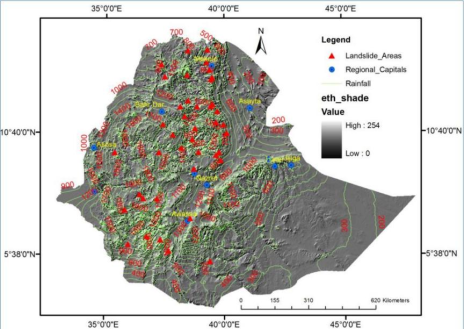
Figure 1. Locations of landslide affected areas in the highlands of Ethiopia.
Numerous landslides have occurred between Km 32+120 and Km 33+200 due to weak geological materials, heavy rainfall, and groundwater shifts, worsened by poor excavation. This study investigates the causes through seismic refraction, Vertical Electrical Sounding (VES), and Electrical Resistivity Tomography (ERT) surveys to develop practical stabilization strategies and mitigate slope failure risks .
With the Limit Equilibrium Method and the Rocscience SLIDE software, the study seeks to assess slope stability under current and prospective unfavorable circumstances . This study evaluates the effectiveness of solutions such as drainage systems, slope re-profiling, and structural reinforcements to enhance road stability. It aims to identify optimal remedial strategies for failed slopes and emphasizes the need for integrated geotechnical analysis and adaptive designs in landslide-prone infrastructure projects within sensitive geological settings.
2. Project Location and Methods of Investigation
For the Masha-Alemtena-Teppi Road Project, a methodical approach was used to investigate the reasons behind slope instability and suggest corrective actions for the crucial landslide-prone areas. To guarantee a thorough grasp of the geotechnical conditions and failure causes, the methodology included literature reviews, field research, laboratory testing, and slope stability analysis.
2.1. Project Location
To gather and examine the information that was already available on the project area, the inquiry started with a thorough desk study. Among them were Examining geological maps, topographic maps, and structural information to find possible geological and geomorphological risks . Figure 2 shows the location map of the area. To determine the size, frequency, and causes of slope failures, historical records of landslides in the area are evaluated . Conducting reconnaissance site visits to observe surface conditions, locate critical areas, and plan detailed field investigations.
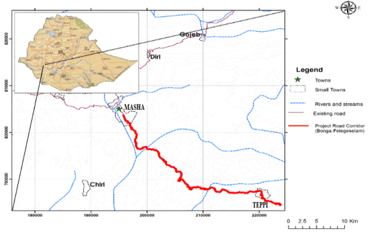
Figure 2. Location Map of the Project Area.
2.2. Physiographic Setting
Rough volcanic, mountainous environment with high to low relief hills is what defines the research region. The elevation above sea level varies between 1718 and 2690 meters. The project region is in the East African Rift System's Broadly Rifted Zone (BRZ), which is in southern Ethiopia . As seen in Figure 3 the geomorphic setting of the region along the route corridor is dominated by plane lands and neighboring highlands. This setting is mostly controlled by internal (tectonic and volcanic) and external forces activities that took place one after the other throughout the previous geological epoch.
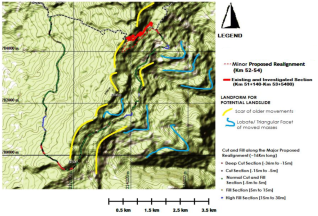
Figure 3. The road project area's landform map.
The construction of Ethiopian rift valleys is associated with tectonic activity, and the main force behind the development of the valley, the nearby highlands, and the isolated hills was volcanic activity in the area . External action is also responsible for the formation of the Gorge system, which ultimately divides the region into valleys where the primary river drainage pattern flows. Because of this, the relief along the route corridor is made up of two distinct types of landforms: mountainous and gorge landforms, and escarpment and flat to rolling landforms, which comprise most of the terrain. Figure 4 illustrates the physiography of the area.
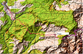
Figure 4. Physiography map of the project region in two-dimensional view.
2.3. Climate and Vegetation
The project area in the Southern Ethiopian highlands experiences a warm, humid subtropical climate with an annual rainfall of approximately 2075 mm (2022–2023) and summer highs around 20°C. Rainfall peaks in July–September and April–May, causing maximum stream flow during winter. The terrain, located between 2050- and 270-meters elevation, falls within the Weina-Dega climatic zone. It features diverse vegetation, including native and introduced trees, with forested highlands dominating the landscape across the road alignment. The three stations' combined temperature data was displayed in Table 1 below.
Table 1. Temperature distribution data of the area.

Location

Jan

Feb

Mar

Apr

May

June

July

Aug

Sept

Oct

Nov

Dec

Masha Station

22.8

24.3

22.8

22.2

21.7

20.8

19.8

19.8

20.5

20.2

22.2

22.8

Alemtena Station

18.2

20.8

21.5

21.5

20.6

20.5

20.6

20

20.5

20.1

20.9

19.5

Teppi Station

18.5

19.6

18.6

18.5

17.3

15.5

15.4

15.5

16.2

17.4

19

20.2

The numbers clearly show that the average temperature in the project area ranges from 15.4 to 24.3. Significant rainfall occurred in 2022 and 2023 between April and October (1864 mm and 1694 mm, respectively).
2.4. Groundwater Conditions
Landslides between Km 32+120 and Km 33+200 occurred at the interface of weathered rock and overlying fragmented soil. Boreholes indicate groundwater depths of 5–13 meters. Springs, visible at topographic breaks, flow year-round with variable discharge, contributing to pore pressure and slope instability in the affected zone. During heavy rainfall, the spring discharge increases, raising pore water pressure within the soil Figure 5 shows spring water indication at km 32+130. The soil bulk is weakened by this high pressure, making it more prone to slide. Slope instability and mass movement in the region are caused by the interaction of shallow groundwater, spring activity, and rainfall-induced pore pressure.
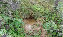
Figure 5. Groundwater/spring water indication at km 32+130.
2.5. Field Investigation
To describe the geology and underlying conditions, a mix of comprehensive geophysical surveys and subsurface exploration was carried out.
2.5.1. Geophysical Surveys
To image the subsurface and offer specific geotechnical features of locations chosen for civil engineering construction, geo-physical approaches have grown in importance . Their cost-effectiveness and ability to continuously provide an overview of the lithology beneath the anticipated structures (i.e., thickness, depth from the ground surface, and other physical attributes of materials) make them desirable. Three distinct techniques were selected for geophysical research, including seismic investi-gation, vertical electrical sounding (VES), and electrical resistivity tomography (ERT) . Figure 6 shows one of the instru-ments used for geophysical investigation for the study given.
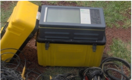
Figure 6. SmartSeis of Geometrix of USA for seismic refraction survey.
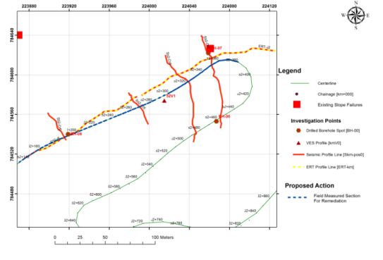
Figure 7. Subsurface exploration details at Km 32+120 to Km 32+280.
Seismic refraction was almost perpendicular to the electrical profiles and ERT because of topographic imperfections in some areas. The purpose of both studies was to map the subsurface geology at specific locations along the Masha-Teppi Road segment, as seen in Figure 7 and Figure 8. To mitigate the impacts of recent landslides between Km 32+120 and Km 33+200, subsurface investigations were conducted to gather geotechnical data. These included seismic refraction spreads, ERT, VES, and boreholes five seismic spreads, one ERT, one VES, and three boreholes at Km 32+120–32+280; and similar setups at Km 32+780–33+200.
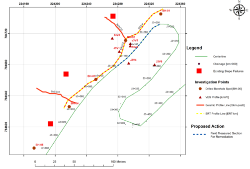
Figure 8. Subsurface exploration details are from Km 32+780 to Km 33+200.
Figure 9 shows that the subsurface underlying line Km 32 is formed of clay, clayey silt, and extensively worn decomposed materials, which are indicated by p-wave velocities below 1500 m/sec and thicknesses between 6 and 18 m. The maximum thickness of the line is little more than eighteen meters at its lowest point, which is at the far NW end.
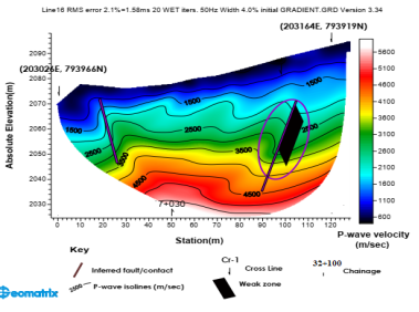
Figure 9. 2D P-wave velocity tomography, road segment Km 32+120.
The 2D-P wave velocity tomography along line Km 32+280 indicates that clay silt and silty clay with gravel are associated with extremely low velocity units that have a thickness of 2.5–12 m and a velocity of 500–1000 m/s. This unit is supported by stiff to hard silty clay and tuff, which have a thickness of 11–17 m and a velocity of 1000–1500 m/sec, Figure 10.
The next unit is interpreted as moderately to slightly fractured basalt (2500- 3500m/s) and is generally situated below 2080m a.s.l Figure 10. The substratum is slightly related to fresh basalt characterized by higher velocities (>3500m/s).
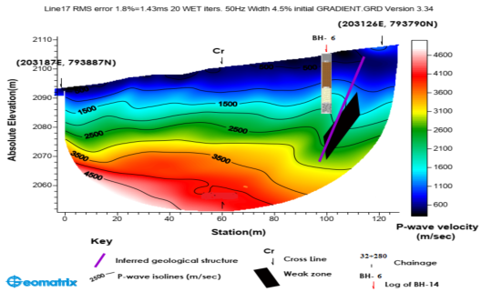
Figure 10. 2D P-wave velocity tomography, road segment Km 32+280.
According to Figure 11, The sloping slope and the southeast-flowing groundwater are likely to result in shallow groundwater and shallow creep because of gravity. The latter is the reason the local embankments have failed. The inferred structure beneath the station and shallow groundwater may also be the primary causes of the fracture around stations 32+340 and the structure extends to about 20m.
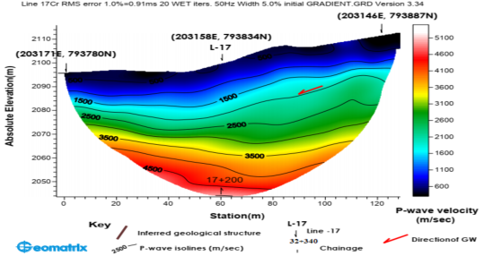
Figure 11. 2D P-wave velocity tomography, across Km 32+340.
The upper portion of the bedrock, which is composed of highly to moderately fractured volcanic rock, most likely rhyolite, is expected to have p-wave velocities in the range of 3000-3500m/sec, with a maximum depth in the central part of the line below ground level (2050m asl), even though there is no borehole log deeper than 20m. Furthermore, fresh bedrock is anticipated to have velocities exceeding 3500 m/sec since rock quality rises with p-wave velocity. Figure 12.
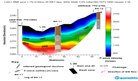
Figure 12. 2D P-wave velocity tomography, Cross Line Cr-500.
2.5.2. Subsurface Exploration
Drilling equipment was used to dig nine boreholes along the impacted areas, which were Km 32+120 to Km 33+200. One of the main tasks was recording data from boreholes, such as descriptions of the rocks and soil, groundwater levels, and the outcomes of in-situ Standard Penetration Tests (SPTs). gathering soil samples for laboratory analysis, both undisturbed and disturbed. Figure 13 illustrates the structural map of the area.
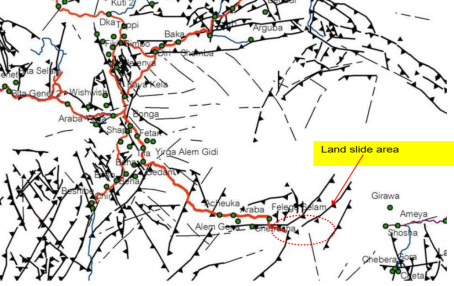
Figure 13. Structural map of landslide and adjacent area modified from Structural map of Teppi area.
2.6. Laboratory Investigation
Samples of rock and soil were chosen with care, and their physical, mechanical, and chemical properties were assessed using extensive laboratory testing . Soil classification involved testing index properties like Liquid Limit (LL), Plastic Limit (PL), and Plasticity Index (PI). Grain size analysis was used to evaluate gradation. Shear strength parameters were determined through Unconfined Compressive Strength, Triaxial Compression, and Direct Shear tests. Moisture content and density tests assessed natural soil conditions.
2.6.1. Geotechnical Characteristics Along Km 32+120-32+225
This portion of the road has a one-bench slope with a 1:1 ratio on the LHS and is situated on a mountain-top plain with rough terrain. Near km 32+180, the cut depth varies from 6 to 10 m, and at km 32+140, it drops to 5 m. While the second bench has dark brown silty clay with up to 70% rock fragments (10–50 cm), the first bench's geology consists of silty clay mixed with boulders of basalt and trachyte. Cracks and downslope creep are obvious indicators of instability. Rock formations, fracture zones, and subsurface water are revealed via seepage and borehole data Table 2 displays the material properties for every layer.
Table 2. Layer properties of station km 32+120- 32+225.

Layer

Thickness

SPT N-Value

Classification (USCS)

PI (%)

LL (%)

Additional Notes

Layer-1

0.0 - 6.50m

6 - 23

ERT

15.5 - 18.75

32.50 - 43.75

Very stiff to hard consistency.

Layer-2

2.0 -17.50m

29 - 42

SC

8.27

24.48

Very dense; significant gravel content.

Layer-3

Extends to 21.75 m

33 - 41

CL

17.16 - 30.59

38.50 - 54.50

Product of altered rhyolite, hard consistency.

2.6.2. Geotechnical Characteristics Along Km 32+300- 32+400
There are cut hills and rugged terrain along the road. While the right-hand side (RHS) has little cutting or is at grade, the left-hand side (LHS) features two benches with a 1:1 ratio that reach a maximum height of 12m at km 32+320.
During a site visit, regressing tension cracks, vertical displacements, and movements were seen between km 32+275 and 32+280 as shown in Figure 14, Figure 15 and Figure 16.
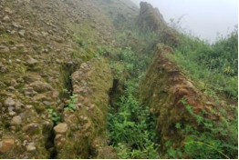
Figure 14. Tension cracks seen between km 32+275 and 32+280.
Table 3. Layer properties of station km 32+300- 32+400.

Layer

Thickness

SPT N-Value

Classification (USCS)

PI (%)

LL (%)

Additional Notes

Layer-1

0.00 - 9.00 m

6 - 50

CL

17.92 - 19.25

37.50 - 38.50

Very stiff to hard consistency.

Layer-2

9.00 - 11.00 m

N/A

SC

21.25

46.25

Contains some gravel.

Layer-3

11.00 -16.70 m

8 - 71

CL

17.39

39.25

Stiff to hard consistency, altered rhyolite.

Layer-4

N/A

N/A

N/A

N/A

N/A

Highly weathered basalt.

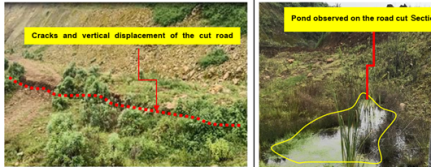
Figure 15. Cracks observed and water ponds in the given station.
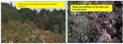
Figure 16. Cracks observed and water ponds in the given station.
During the wet season, these fissures could get worse and impact the local slope. Water infiltration from the LHS pond interacts with spoil materials put on the LHS between km 32+200 and 32+300, seeps into roadbed fissures, and exits on the RHS as seepage. The RHS becomes unstable because of the spoil being saturated by this surface and subsurface water. The road failures were linked to unregulated spoil disposal, which was not noticed during the site visit, according to investigations. Particularly during the wet season, this condition may result in severe cracking and sliding. Table 3 shows the characteristics of each soil layer of the given location.
Table 4. Layer properties of station km 32+400-32+900.

Layer

Thickness

SPT N-Value

Classification (USCS)

Unit Weight (KN/m3)

C (KN/m2)

Φ (°)

Layer-1

0.0 - 10.0 m and 14.0 - 18.0 m

3.0 - 27 (top), 48 - 65 (bottom)

CL

8.19

38

50

Layer-2

10.0 - 14.0 m

15 - 50

SC

N/A

N/A

N/A

Layer-3

Extends to 18.0 m

Ended with 50 (refusal)

GC

18.29

24

25

Layer-4

Extends to 28.0 m

N/A

N/A

N/A

N/A

N/A

2.6.3. Geotechnical Characteristics Along Km 33+100-33+200
During the wet season, water from a pond on the left-hand side infiltrates and saturates spoil materials placed between Km 32+200 and 32+300. This moisture seeps into existing roadbed fissures and reemerges on the right-hand side, leading to reduced slope stability. The situation is worsened by unregulated spoil disposal, which was overlooked during site inspections. As a result, the combination of saturated spoil and poor drainage significantly increases the risk of cracking and landslides.
Table 5. Layer properties of station km 33+100-33+200.

Layer

Depth (m)

SPT N Value

USCS Classification

Plasticity Index (PI, %)

Layer-1

6.0-6.85 borehole-1 (BH-1), 6.0-17.0 (BH-1A), 0.0-2.0 (BH-2)

11-50

CL

21.03

Layer-2

0-6 (BH-1), 0-3 (BH-1A), 2.0-17.5 (BH-2)

6-26

CL with some gravel

18.24-31.96

Layer-3

3-6, 17.0-20.0 (BH-1A)

16-50

CL, CH (top part with some gravel)

Not specified

Layer-4

8.5-15.0 (BH-1), 17.5-29.0 (BH-2)

27-80

CL (sandy lean clay)

20.83-20.86

3. Slope Stability Analysis
Subsurface profile using geophysical surveys and borehole data, interpreted for worst-case scenarios, served as the foundation for the slope stability analysis . Laboratory and in-situ experiments were used to assess the soil's characteristics, such as its shear strength, dry and saturated unit weights, and categorization outcomes. Under effective pore pressure circumstances, the factor of safety (FS) was computed using a pore fluid unit weight of 9.81 kN/m3 for full saturation. Based on field observations, it was predicted that the slump failure would rotate and have a circular surface that extended from the cut surface or slope height to the road drainage's toe.
3.1. Landslides at Km 32+120 to 32+225
There is no discernible mass movement in this area, which shows indications of instability in the form of downslope creep and a sizable crack at the top of the cut portion that extends about three meters. Geophysical surveys and drilling studies verified the discovery of seepage signs at km 32+140 at the bottom portion. Additionally, the geometry, slope mass profile (for both the current and designed cuts), material properties, and groundwater conditions between km 32+120 and 32+225 are detailed illustrated in Table 6 and Figure 17.
Table 6. Material data of the soil profile at km 32+120 and 32+225.

Material Type

Unit Weight (KN/m3)

Cohesion (KN/m²)

Friction Angle (°)

Groundwater Table Ref.

Lean Clay (CL)

18.75

37

17

Partially Below

Clayey Sand (SC)

18.45

24

12

Below

Stiff Lean Clay

18.43

36

53

Below

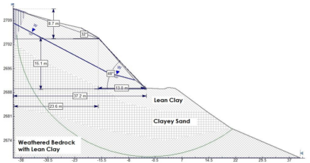
Figure 17. Representative section of the current cut condition at Km 32+200.
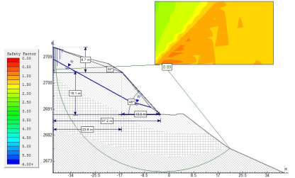
Figure 18. Slope stability status at the current cut condition shows instability.
3.2. Back Slope Failure at Km 32+300 to 32+400
There is erratic vertical displacement and lateral movement in this portion of the cut slope, especially between the dumped spoil material and the road cut edge. During a site visit, these problems were noted between Km 32+355 and Km 32+380. Significant fractures and slip failures were caused by water infiltration that was observed from the left-hand side (LHS) of a neighboring pond. Additionally, the geometry, slope mass profile, material properties, and groundwater conditions for the section between Km 32+355 and Km 32+380 are detailed in Table 7 and Figure 19.
Table 7. Material data of the soil profile at km 32+300 to 32+400.

Soil Type

Unit Weight (kN/m3)

Cohesion (kN/m²)

Friction Angle (°)

Groundwater Table Reference

Lean Clay [CL]

20.65

35

18

Partially below

Clayey Sand [SC]

19.55

23

15

Below

Stiff Lean Clay

18.73

37

51

Below

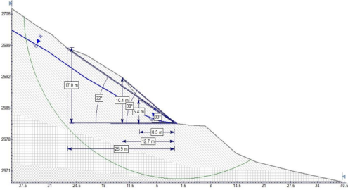
Figure 19. Representative section of the current cut condition at Km 32+360.
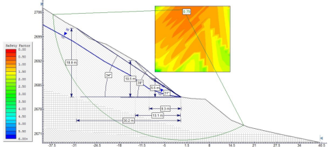
Figure 20. Slope stability status at the current cut condition at Km 32+360.
As seen in Figure 20 final design cut shows instability defined by 0.79 factor of safety indicating its potential to fail in full saturation.
3.3. Landslide at Km 32+400 to 32+900 (LHS)
Significant sliding has occurred in this region, with motions simulating an earth flow stretching about two hundred meters southwest near Km 33+000. According to field studies, the area's springs are mostly the result of topographic cracks and are frequently located where colluvial material meets the underlying rock. The geometry, slope mass profile, material properties, and groundwater conditions for the section between Km 32+400 and Km 32+900 are detailed Table 8 and Figure 21.
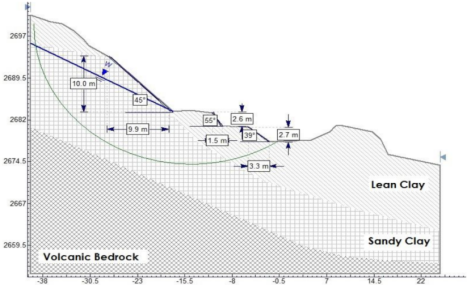
Figure 21. Representative section of the current cut condition at Km 32+400.
Table 8. Material data of the soil profile at km 32+400 to 32+900 (LHS).

Soil Type

Unit Weight (kN/m3)

Cohesion (kN/m²)

Friction Angle (°)

Groundwater Table Reference

Lean Clay [CL]

18.23

29

27

Partially below

Sandy Clay [SC]

17.86

32

55

Below

Volcanic Bedrock

UCS – 5 MPa with GSI= 50

Below

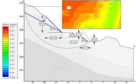
Figure 22. Slope stability status at the current cut condition at Km 32+400.
Slope stability status at the current cut condition and final design cut is showing a contrasting instability defined by 0.56 factor of safety as shown in Figure 22 indicating it’s unstable at current condition, but further cut might not induce further instability; rather it seems it is already exhausted.
3.4. Landslide at Km 33+100 to 33+200
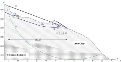
Figure 23. Representative section of the current cut condition at Km 33+140.
Only the left-hand side (LHS) slope is affected by the failure in this segment. A landslide can be caused by deep water infiltration into the transported and residual clays and gravel layers, which is made possible by colluvial deposits. On the LHS slope, seepage was noted near the junction of clay-mixed boulders and broken rock. The geometry, slope mass profile, material properties, and groundwater conditions for the section between Km 33+100 and Km 33+200 are outlined Table 9 and Figure 23.
Table 9. Material data of the soil profile at km 33+100 to 33+200 (LHS).

Soil Type

Unit Weight (kN/m3)

Cohesion (kN/m²)

Friction Angle (°)

Groundwater Table Reference

Lean Clay [CL]

18.80-18.91

35-42

18-53

Partially below

Volcanic Bedrock

UCS – 5 MPa with GSI= 50

Below

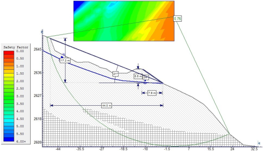
Figure 24. Slope stability status at the current cut condition at Km 33+140.
Additionally, the final design cut exhibits instability as indicated by the 0.76 factor of safety, meaning that it is unstable as it is and will become even more unstable with additional cuts.
4. Sensitivity and Back Analysis
4.1. Sensitivity Analysis
Table 10. The results for the slope stability analysis in different instable sections.

Instable stretch (km)

Representative section (km)

Factor of safety current cut status

32+120-32+225

32+200

0.89

32+300-32+400

32+360

0.79

32+400-32+900

32+400

0.56

33+100-33+200

33+140

0.76

Sensitivity analysis was used to evaluate the effects of significant variables on slope stability, such as cohesion, internal fric-tion angle, and groundwater levels . Back analysis was performed on sections with recorded failures to confirm input pa-rameters and enhance the models .
The specifications for slope cut strength to do the sensitivity analysis and investigate the effect on the safety parameters, the cohesiveness and friction angle were changed . This investigation employed the Janbu approach, which involved separate-ly adjusting each of the parameters as indicated in For slope cut situations, the ERA manual defines a factor of safety of <1, which indicates failure, 1.0-1.5 as dubious safety, and >1.5 as safe .
To indicate stability conditions based on ERA cut slope design, the values utilized for cohesion and friction angles increased by 25%, 50%, 75%, and 100% until the factor of safety had risen over 1.5 . For slope cut situations, the ERA manual de-fines a factor of safety of <1, which indicates failure, 1.0-1.5 as dubious safety, and >1.5 as safe .
Table 11. The results for the sensitivity analysis in variable strength parameters.

Factor of safety

Factor of safety by

Cohesion increment

Angle of friction increment

25%

50%

75%

100%

25%

50%

75%

100%

0.89

0.90

0.91

0.94

0.95

0.94

0.99

1.13

1.18

0.79

0.85

0.91

0.95

1.01

0.88

0.97

1.07

1.2

0.56

0.61

0.7

0.79

0.89

0.71

0.84

0.95

1.13

0.76

0.88

0.96

1.04

1.21

0.92

1.01

1.21

1.35

From the result shown in for slope cut situations, the ERA manual defines a factor of safety of <1, which indicates failure, 1.0-1.5 as dubious safety, and >1.5 as safe .
Table 11 the factor of safety did not get above 1.5 (safe range), in any strength increment. In another set of sensitivity analyses, variable moisture conditions were considered to define the impact of moisture and groundwater saturation as shown in Table 12. Additionally, it was observed that saturations are linked to a few of the clipped parts' failures. For this experiment, three distinct cases full saturation, moderately saturated, and dry state were used to develop the saturation variations.
Table 12. The results for the sensitivity analysis in variable saturation conditions.

Cut section (km)

Factor of safety

Factor of safety

Full saturation

Partially saturated

Dry condition

32+200

0.89

0.51

1.46

2.25

32+360

0.79

0.43

1.31

2.01

32+400

0.56

0.35

1.24

2.72

33+140

0.76

0.59

1.01

2.73

4.2. Back Analysis Results
Table 13. Back analysis for calculation of reinforcement forces.

Cut section (km)

Reinforcement (toe) elevation msal

Active force (kN)

Passive force (kN)

32+200

2683

1567.65

1490.78

32+360

2671

1435.65

1283.48

32+400

2665

1713.5

1870

33+140

2636

1822.97

2197.33

The computed passive forces are those required to boost the resisting forces, which retaining walls can supply . The value of the active forces calculated is the amount needed to be removed from the driving forces to achieve a factor of safety of 1.5.
A back analysis was performed to determine the amount of force required to reinforce the slope cut at the toe, aiming to raise the factor of safety to 1.5 . The analysis's findings will direct the creation of reinforcing structures. To guarantee that the factor of safety reaches acceptable levels (> 1.5), the computed values will help with the design parameters for the structures required to reinforce the cut parts. Both active and passive forces were assessed during the back analysis as shown in Table 13.
4.3. Taguchi Analysis
The Taguchi method is a statistical approach designed to optimize process parameters and improve quality by minimizing variability. In geotechnical engineering, particularly in slope stability analysis, this method has been employed to identify the most influential factors affecting slope stability and to determine optimal conditions for safety and performance.
One notable application of the Taguchi method in slope stability analysis is presented in the study by , This study investi-gated how key soil and geometric parameters affect the stability of homogeneous slopes using the Taguchi method. Five fac-tors bulk density, cohesion, internal friction angle, slope height, and slope length were analyzed at four levels through an L16 orthogonal array. This allowed the assessment of sixteen parameter combinations, reducing experimental runs while maintain-ing analytical depth. Factor of Safety (FoS) was computed for each setup using the ordinary method of slices.
Results showed slope height was the most influential factor (53.2%), followed by slope length and cohesion. The Taguchi approach proved accurate and efficient in predicting slope stability outcomes. Using the Taguchi method, researchers systematically varied input parameters and analyzed displacement data to calibrate their numerical models and identify the most influential factors governing cavern stability. The study demonstrated the Taguchi method’s effectiveness in optimizing parameters for more reliable predictions. Its broader applications in geotechnical engineering such as evaluating soil strength, retaining wall design, and slope stability underscore its versatility in solving complex, multi-variable engineering challenges with minimal experimentation.
4.4. Taguchi Method-based Parametric Optimization
To enhance slope stability analysis beyond traditional limit equilibrium methods, the Taguchi approach was applied to identify and optimize key geotechnical and geometric factors influencing the Factor of Safety (FOS). An L16 orthogonal array was used to assess five critical parameters cohesion, internal friction angle, unit weight, slope height, and groundwater depth each at four levels. FOS values were calculated using SLIDE software under dry and saturated conditions. The signal-to-noise ratio, based on the “larger-the-better” criterion, and ANOVA analysis highlighted the most impactful variables. This integration provided efficient, data-driven insights for designing optimal remedial solutions in failure-prone slope sections.
4.5. Signal-to-Noise (S/N) Ratio Formulas in Taguchi Method
The Signal-to-Noise (S/N) ratio is a measure used in the Taguchi method to evaluate the robustness of a system or design. Depending on the optimization objective, different formulas are used.
1. Larger-the-Better (e.g., maximize Factor of Safety):
Signal-to-Noise Ratio (S/N ratio) = -10 × log₁₀ [(1/n) × Σ (1 / Yᵢ²)] = -10 × log log10[1n ×i=1n (y0 -y1) S/N ratio =
-10 × log₁₀ [1ni=1n(y0-y1)2]
Where:
n = number of observations (usually 1 per trial)
Yᵢ = observed value in the i-th trial
4.6. Main Effect Plots by Section
1) Section 32+200 and 32+260
Figure 25 shows the influence of each parameter on slope stability in Section 32+200 and 32+260. The parameter with the steepest slope and highest S/N ratio has the strongest effect on Factor of Safety.
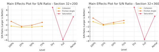
Figure 25. Signal to noise ratio plot for section 32+200 and 32+360.
2) Section 32+400 and 33+140
Figure 26 shows the influence of each parameter on slope stability in Section 32+400 and 33+140. The parameter with the steepest slope and highest S/N ratio has the strongest effect on Factor of Safety.
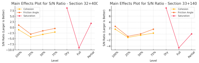
Figure 26. Signal to noise ratio plot for section 32+400 and 33+140.
4.7. ANOVA Results for Taguchi Slope Stability Analysis
Table 14. ANOVA result for each road segment.

Factor

SS

DF

MS

% Contribution

Section

Cohesion

0.132

3

0.044

6.7014

32+200

Friction Angle

0.0469

3

0.0156

2.38

32+200

Saturation

1.7903

2

0.8951

90.9186

32+200

Error

0.0

2

0.0

0.0

32+200

Cohesion

0.0747

3

0.0249

4.9735

32+360

Friction Angle

0.0588

3

0.0196

3.9149

32+360

Saturation

1.3693

2

0.6846

91.1117

32+360

Error

-0.0

2

-0.0

-0.0

32+360

Cohesion

0.2856

3

0.0952

7.3887

32+400

Friction Angle

0.1246

3

0.0415

3.2222

32+400

Saturation

3.4553

2

1.7276

89.3891

32+400

Error

0.0

2

0.0

0.0

32+400

Cohesion

0.151

3

0.0503

4.9292

33+140

Friction Angle

0.1235

3

0.0412

4.0315

33+140

Saturation

2.7897

2

1.3948

91.0393

33+140

Error

0.0

2

0.0

0.0

33+140

In all sections, the Saturation factor contributed most significantly to slope stability variations, emphasizing the need for effective groundwater and drainage management in landslide-prone regions.
This section presents the ANOVA results for each road segment analyzed using the Taguchi method as seen in Table 14. The table below summarizes the sum of squares (SS), degrees of freedom (DF), mean square (MS), and percentage contribution of each factor toward the variation in Factor of Safety (FOS).
4.8. Taguchi Analysis Integration
The implementation of the Taguchi method provided valuable insights into the parametric sensitivity of slope stability along four critical failure sections of the Masha-Alemtena-Teppi Road. An L9 orthogonal array was used to evaluate the effects of cohesion, internal friction angle, and saturation on the computed Factor of Safety (FOS). Main effect plots and S/N ratio analyses revealed that saturation was the most influential factor affecting slope stability, as evidenced by the steep slope of its response curves across all sections.
ANOVA further quantified the relative impact of each parameter. Saturation accounted for over 90% of the total variance in all sections, with specific contributions of 90.9%, 91.1%, 89.4%, and 91.0% for sections 32+200, 32+360, 32+400, and 33+140, respectively. Friction angle and cohesion contributed marginally, with average effects below 7%. These findings highlight that minor variations in groundwater conditions or moisture content can significantly alter the stability of cut slopes, even when soil strength parameters remain constant.
The predictive robustness of the Taguchi method, combined with its efficiency in reducing simulation trials, demonstrated its suitability for rapid parametric screening. Its results align closely with field observations and traditional limit equilibrium outcomes, reinforcing its reliability. Importantly, this analysis supports the prioritization of groundwater control strategies such as drainage trenches, underdrains, and surface water diversion as central components of slope stabilization in similar geologically sensitive terrains.
5. Development of Remedial Measures
To address slope instability, site-specific corrective actions were suggested considering the findings. Re-profiling the slopes into more stable shapes, putting in surface and subsurface drainage systems to control water infiltration, strengthening the slopes with retaining walls and soil nails, and stabilizing the surface layers with vegetation and erosion control methods were all part of these measures .
5.1. Remedial Measure Between Km 32+120 and Km 32+220
The slope segment between Km 32+120 and Km 32+225 is unstable based on current and final cut evaluations. Recommended remedial measures include removing loose rock and soil from the lower bench to match the upper slope’s angle, thereby stabilizing gradients, and reducing water infiltration. Surface re-grading is advised to eliminate depressions and reshape the landslide head scarp. A multi-layer gabion wall should be constructed at the toe, supported by rock backfill at a 1:2 batter slope as shown in Figure 27. Additional measures include installing crest drainage, vegetating the slope face, capturing subsurface water, and constructing a paved side ditch along the LHS.
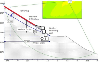
Figure 27. Stability analysis with the recommended remedial at 32+200 km.
5.2. Remedial Measure Between Km 32+300 and Km 32+400 on the LHS
The slope between Km 32+300 and 32+400 is unstable, with a factor of safety of 0.79. To stabilize it, landslide debris and weakened materials must be removed and replaced with compacted rock fill and granular layers. A 1.5–2 meter retaining wall and underdrain on the LHS are also recommended. The slope stability study indicates an enhanced factor of safety of 2.19 with these precautions in place, as illustrated in Figure 26.
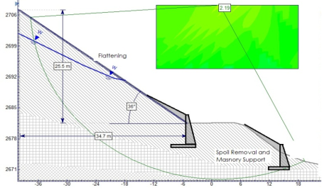
Figure 28. Stability analysis with the recommended remedial at 32+360 km.
5.3. Remedial Measure Between Km 32+400 and Km 32+900
To stabilize the slide zone, all unstable soil must be removed from both the top and bottom, starting from the upper slope to reduce driving forces. A retaining wall should then be constructed on solid bedrock, accounting for potential groundwater rise. The design must include weep holes with geosynthetic filters, and an underdrain should be installed behind the wall to manage subsurface flow. A cascade system is also recommended to redirect spring water into the roadside drainage channel. It is anticipated that these actions will increase slope stability and result in a factor of safety of at least 2.36, as illustrated in Figure 27.
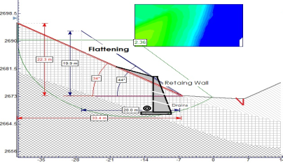
Figure 29. Stability analysis with the recommended remedial at km 32+400.
5.4. Remedial Measure Between Km 33+100 and Km 33+200
It is advised that all sliding soil materials be removed from the upper and lower portions of the slide region to the necessary level in this section. To lessen the driving force and stop sliding, material should be removed starting at the top and working its way down.
Following the recommended foundation depth, a retaining wall should be built on competent and stable bedrock between km 33+100 and 33+200 on the LHS once the slide materials have been cleared. On the LHS of the road, behind the retaining wall, an underdrain should be placed to control subsurface water. It will divert water to the closest drainage structure. These measures are expected to improve slope stability, achieving a factor of safety of 1.93, as illustrated in Figure 28.
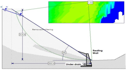
Figure 30. Stability analysis with the recommended remedial at 33+140 km.
6. Conclusion
This study integrated geotechnical field data, limit equilibrium modeling, and the Taguchi method to assess slope stability along critical sections of the Masha-Alemtena-Teppi Road. While traditional analyses confirmed instability under current and saturated conditions, Taguchi optimization revealed that groundwater saturation was the dominant factor influencing failure, contributing over 90% to FOS variation across all sections. Friction angle and cohesion had lesser impacts. The findings support prioritizing drainage and moisture control strategies in remediation. This combined approach enhances understanding of slope failure mechanisms and offers a replicable, data-efficient framework for designing resilient infrastructure in landslide-prone environments.
Abbreviations

ANOVA

Analysis of Variance

BRZ

Broadly Rifted Zone

CL

Lean Clay (Unified Soil Classification System)

CH

High Plasticity Clay (Unified Soil Classification System)

ERT

Electrical Resistivity Tomography

FOS/FS

Factor of Safety

GSI

Geological Strength Index

GC

Clayey Gravel (Unified Soil Classification System)

GIS

Geographic Information System

LHS

Left-Hand Side

LL

Liquid Limit

L9/L16

Taguchi Orthogonal Array with 9 / 16 Experiments

PL

Plastic Limit

PI

Plasticity Index

RHS

Right-Hand Side

S/NRatio

Signal-to-Noise Ratio

SC

Clayey Sand (Unified Soil Classification System)

SLIDE

Rocscience SLIDE Slope Stability Software

SPT

Standard Penetration Test

UCS

Unconfined Compressive Strength

USCS

Unified Soil Classification System

VES

Vertical Electrical Sounding

Author Contributions
Aklilu Shitu: Investigation, Data curation, Methodology, Software, Formal analysis, Writing – original draft.
Ermias Shitu: Supervision, Formal analysis, Writing – original draft
Conflicts of Interest
The authors declare no conflicts of interest.
References
[1] D. V. &. F. G. A. Griffiths, Probabilistic Methods in Geotechnical Engineering (CISM Courses and Lectures, Vol. 491), Springer, 2007.
[2] F. M. N. &. M. F. Sengani, “Establishing reliable slope stability hazard map based on GIS-based tool in conjunction with finite element methods,” Advances in Civil Engineering, pp. 2022, 3384143, 2022.
[3] K. B. L. M. L. &. W. S. Y. Sim, “A review of landslide acceptable risk and tolerable risk.,” Geoenvironmental Disasters, pp. 9, 3., 2022.
[4] Y. M. &. L. C. K. Cheng, Slope Stability Analysis and Stabilization: New Methods and Insight., CRC Press/Taylor & Francis., 2008.
[5] K. Woldearegay, “Characteristics of landslides affecting road networks in Ethiopia: Evidence from 25 years research, practice and documentation.,” in Progress in Landslide Research and Technology, vol. 3, Springer Nature, 2025.
[6] P. T. G. H. S. &. A. E.-R. A. Imani, “Application of combined electrical resistivity tomography (ERT) and seismic refraction tomography (SRT) to investigate Xiaoshan District landslide: Hangzhou, China.,” Journal of Applied Geophysics, pp. 184, 104236., 2021.
[7] D. Q. S. H. I. S. H. B. S. M. M. S. F. I. &. I. M. Kazmi, “Slope remediation techniques and overview of landslide risk management.,” Civil Engineering Journal, pp. 3(3), 180–189., 2017.
[8] A. B. M. C. C. P. G. R. E. &. S. M. J. Chelli, “Geomorphological tools for mapping natural hazards.,” Journal of Maps, pp. 17(3), 265–279., 2021.
[9] A. C. C. M. D. S. E. R. B. B. P. H. S. M. R. Erbello, “Magma-assisted continental rifting: The Broadly Rifted Zone in SW Ethiopia, East Africa.,” Tectonics, pp. 43(1), e2022TC007651, 2024.
[10] L. &. S. O. Schrott, “Application of field geophysics in geomorphology: advances and limitations exemplified by case studies.,” Geomorphology, pp. 93(1–2), 55–73., 2008.
[11] M. Z. Z. G. W. P. T. &. W. M. Zou, “Analysis of typical rock physical characteristics, mechanical properties, and failure modes of the Laoheba Phosphate Mining Area in the Sichuan Basin, China.,” Lithosphere, p. 2023_348, 2024.
[12] A. B. P. B. M. D. M. H. J. C. T. &. B. R. Bichler, “Three-dimensional mapping of a landslide using a multi-geophysical approach: the Quesnel Forks landslide, British Columbia, Canada.,” Landslides, pp. 1, 29–40., 2004.
[13] C. &. S. S. Meisina, “A comparative analysis of terrain stability models for predicting shallow landslides in colluvial soils.,” Geomorphology, pp. 87(3), 207–223., 2007.
[14] R. D. A. &. B. V. Nassirzadeh, “Back analysis of cohesion and friction angle of failed slopes using probabilistic approach: two case studies.,” International Journal of Geo-Engineering, pp. 15, 3., 2024.
[15] K. M. G. Y. B. V. R. K. &. S. Z. Bushira, “Cut soil slope stability analysis along National Highway at Wozeka–Gidole Road, Ethiopia.,” Modeling Earth Systems and Environment, pp. 4(2), 591–600, 2018.
[16] Ö. Tan, “Investigation of soil parameters affecting the stability of homogeneous slopes using the Taguchi method.,” Eurasian Soil Science, pp. 39(11), 1248–1254., 2006.
[17] L. A. M. &. S. X. Fay, Cost-Effective and Sustainable Road Slope Stabilization and Erosion Control (NCHRP Synthesis 430)., Transportation Research Board., 2012.
Cite This Article
  • APA Style

    Shitu, A., Shitu, E. (2026). Utilizing the Taguchi Method to Optimize Slope Stability and Analyse Parameter Sensitivity in Road Cuts: Insights from Southern Ethiopia. Science Discovery Environment, 1(1), 33-54. https://doi.org/10.11648/j.sdenv.20260101.14

    Copy | Download

    ACS Style

    Shitu, A.; Shitu, E. Utilizing the Taguchi Method to Optimize Slope Stability and Analyse Parameter Sensitivity in Road Cuts: Insights from Southern Ethiopia. Sci. Discov. Environ. 2026, 1(1), 33-54. doi: 10.11648/j.sdenv.20260101.14

    Copy | Download

    AMA Style

    Shitu A, Shitu E. Utilizing the Taguchi Method to Optimize Slope Stability and Analyse Parameter Sensitivity in Road Cuts: Insights from Southern Ethiopia. Sci Discov Environ. 2026;1(1):33-54. doi: 10.11648/j.sdenv.20260101.14

    Copy | Download

  • @article{10.11648/j.sdenv.20260101.14,
      author = {Aklilu Shitu and Ermias Shitu},
      title = {Utilizing the Taguchi Method to Optimize Slope Stability and Analyse Parameter Sensitivity in Road Cuts: Insights from Southern Ethiopia},
      journal = {Science Discovery Environment},
      volume = {1},
      number = {1},
      pages = {33-54},
      doi = {10.11648/j.sdenv.20260101.14},
      url = {https://doi.org/10.11648/j.sdenv.20260101.14},
      eprint = {https://article.sciencepublishinggroup.com/pdf/10.11648.j.sdenv.20260101.14},
      abstract = {Slope instability represents a major challenge for road infrastructure in mountainous regions, particularly where complex geology, intense rainfall, and shallow groundwater prevail. The Masha–Alemtena–Teppi Road corridor in southern Ethiopia has experienced recurrent slope failures that threaten public safety and infrastructure performance. This study investigates the failure mechanisms along critical road sections and identifies the most influential parameters governing slope stability. An integrated approach combining geotechnical field investigations, laboratory testing, geophysical surveys, and numerical slope stability modeling was adopted. Limit equilibrium analyses were performed using Rocscience SLIDE software to compute the Factor of Safety (FOS) under existing, saturated, and design cut conditions. The results show that current FOS values range from 0.56 to 0.89, indicating unstable to critically unstable slopes. Sensitivity analysis revealed that increasing cohesion or friction angle by up to 100% was insufficient to raise FOS above the safe threshold of 1.5, whereas groundwater conditions had a pronounced effect. Under dry conditions, FOS values increased to 2.01–2.73, while full saturation reduced FOS to as low as 0.35–0.59. To quantitatively assess parameter influence, the Taguchi method was applied using an L9 orthogonal array with cohesion, internal friction angle, and saturation as control factors. Signal-to-noise ratio analysis and analysis of variance (ANOVA) results indicate that saturation accounts for 89–91% of FOS variation across all sections, while cohesion and friction angle contribute less than 7% each. Back analysis estimated required reinforcement forces ranging from 1,283 to 2,197 kN to achieve a target FOS of 1.5. Based on these findings, site-specific remedial measures, including drainage systems, slope re-profiling, and retaining structures—were proposed, resulting in improved FOS values of up to 2.36. The study demonstrates that integrating statistical optimization with conventional geotechnical analysis provides a robust and efficient framework for slope stability assessment and mitigation design in landslide-prone regions.},
     year = {2026}
    }
    

    Copy | Download

  • TY  - JOUR
    T1  - Utilizing the Taguchi Method to Optimize Slope Stability and Analyse Parameter Sensitivity in Road Cuts: Insights from Southern Ethiopia
    AU  - Aklilu Shitu
    AU  - Ermias Shitu
    Y1  - 2026/02/06
    PY  - 2026
    N1  - https://doi.org/10.11648/j.sdenv.20260101.14
    DO  - 10.11648/j.sdenv.20260101.14
    T2  - Science Discovery Environment
    JF  - Science Discovery Environment
    JO  - Science Discovery Environment
    SP  - 33
    EP  - 54
    PB  - Science Publishing Group
    UR  - https://doi.org/10.11648/j.sdenv.20260101.14
    AB  - Slope instability represents a major challenge for road infrastructure in mountainous regions, particularly where complex geology, intense rainfall, and shallow groundwater prevail. The Masha–Alemtena–Teppi Road corridor in southern Ethiopia has experienced recurrent slope failures that threaten public safety and infrastructure performance. This study investigates the failure mechanisms along critical road sections and identifies the most influential parameters governing slope stability. An integrated approach combining geotechnical field investigations, laboratory testing, geophysical surveys, and numerical slope stability modeling was adopted. Limit equilibrium analyses were performed using Rocscience SLIDE software to compute the Factor of Safety (FOS) under existing, saturated, and design cut conditions. The results show that current FOS values range from 0.56 to 0.89, indicating unstable to critically unstable slopes. Sensitivity analysis revealed that increasing cohesion or friction angle by up to 100% was insufficient to raise FOS above the safe threshold of 1.5, whereas groundwater conditions had a pronounced effect. Under dry conditions, FOS values increased to 2.01–2.73, while full saturation reduced FOS to as low as 0.35–0.59. To quantitatively assess parameter influence, the Taguchi method was applied using an L9 orthogonal array with cohesion, internal friction angle, and saturation as control factors. Signal-to-noise ratio analysis and analysis of variance (ANOVA) results indicate that saturation accounts for 89–91% of FOS variation across all sections, while cohesion and friction angle contribute less than 7% each. Back analysis estimated required reinforcement forces ranging from 1,283 to 2,197 kN to achieve a target FOS of 1.5. Based on these findings, site-specific remedial measures, including drainage systems, slope re-profiling, and retaining structures—were proposed, resulting in improved FOS values of up to 2.36. The study demonstrates that integrating statistical optimization with conventional geotechnical analysis provides a robust and efficient framework for slope stability assessment and mitigation design in landslide-prone regions.
    VL  - 1
    IS  - 1
    ER  - 

    Copy | Download

Author Information
  • Abstract
  • Keywords
  • Document Sections

    1. 1. Introduction
    2. 2. Project Location and Methods of Investigation
    3. 3. Slope Stability Analysis
    4. 4. Sensitivity and Back Analysis
    5. 5. Development of Remedial Measures
    6. 6. Conclusion
    Show Full Outline
  • Abbreviations
  • Author Contributions
  • Conflicts of Interest
  • References
  • Cite This Article
  • Author Information