Abstract
Dead-end pores are important microstructural features in porous media because they strongly influence flow efficiency, transport behaviour, and solute retention. However, their identification remains challenging due to geometric complexity and the limitations of conventional post-processing methods. In this study, we developed a machine-learning framework for the automated prediction of dead-end pores from pore-scale velocity-field data obtained through numerical fluid-flow simulations. Two-dimensional and three-dimensional porous geometries were constructed using CAD tools and simulated under Stokes and Navier-Stokes flow regimes using the CSMP platform. The resulting pressure and velocity fields were exported in Visualization Toolkit (VTK) format, and spatial as well as hydrodynamic features were extracted for analysis. A supervised classification approach based on a Random Forest model was trained on 222,810 pore-scale data points, using spatial coordinates and pressure as predictor variables. Dead-end pores were defined as stagnant regions weakly connected to the main flow pathways and labelled accordingly. Model performance was evaluated using accuracy, precision, recall, and ROC-AUC, along with three-dimensional visualizations for physical validation. The proposed model achieved an accuracy of 98.20%, a recall of 96.19% for dead-end pore identification, and a ROC-AUC score of 0.9985, indicating excellent predictive performance and robustness. These results show that machine learning can reliably distinguish active flow channels from stagnant dead-end regions directly from velocity-field data without explicit connectivity analysis. The approach offers a scalable and objective tool for pore-scale characterization with potential applications in enhanced oil recovery, contaminant transport, and digital rock physics.
Keywords
Dead-end Pores, Random Forest Classifier, Velocity-field Data, Digital Rock Physics, Enhanced Oil Recovery,
Visualization Toolkit (VTK)
1. Introduction
Fluid flow through porous media is a fundamental phenomenon in a wide range of natural and engineered systems, including groundwater transport, hydrocarbon recovery, fuel cell design, and filtration processes. The intricacy of flow behavior in such systems is largely governed by the geometric and topological heterogeneity of the pore structure. Among the micro-structural features that significantly influence flow and transport processes, dead-end pores play a particularly important role. Dead-end pores, also referred to as stagnant or blind-end pores, are cavities connected to the main pore network at only one end
| [1] | Bijeljic, B., Mostaghimi, P., & Blunt, M. J. (2013). Insights into non-Fickian solute transport in carbonates. Water Resources Research, 49(5), 2714-2728. |
[1]
. In these regions, fluid can enter but does not actively take part in advective flow, thereby resulting in locally stagnant zones that contribute minimally to through-flow. Consequently, dead-end pores may serve as solute storage regions, promoting prolonged residence times, diffusion-dominated transport, and incomplete fluid displacement
| [2] | Valvatne, P. H., & Blunt, M. J. (2004). Predictive pore-scale modeling of two-phase flow in mixed wet media. Water Resources Research, 40(7). |
| [3] | Andrew, M., Bijeljic, B., & Blunt, M. J. (2014). Pore-scale imaging of trapped carbon dioxide in sandstones and carbonates. International Journal of Greenhouse Gas Control, 22, 1-14. |
[2, 3]
.
The presence of dead-end pores has significant implications for the hydrodynamic and the reactive properties of porous systems. For example, they can largely reduce the effective permeability, increase tortuosity, and alter mass transfer rates between flowing and stagnant regions
| [4] | Soulaine, C., Gjetvaj, F., & Tchelepi, H. A. (2021). Pore-scale description of multiphase flow in porous media: Revisiting the role of the wetting phase. Transport in Porous Media, 140(1), 1-26. |
[4]
. These effects are relevant in applications such as enhanced oil recovery, contaminant transport, and catalytic reactor design, where flow efficiency and solute exchange strongly influence performance
| [3] | Andrew, M., Bijeljic, B., & Blunt, M. J. (2014). Pore-scale imaging of trapped carbon dioxide in sandstones and carbonates. International Journal of Greenhouse Gas Control, 22, 1-14. |
[3]
. The accurate identification and quantification of dead-end pores are therefore essential for predictive modeling and for the design of porous materials with optimized flow properties.
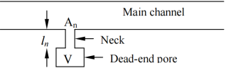
Figure 1. Illustration of dead-end pore in porous media (Muhammad et al, 2008).
Figure 1 illustrates the dead-end pore model in a porous medium as employed by the works of
Goodknight et al. (1960) and
Fatt et al. (1966). The model consists of a neck and a body, with the neck much narrower than the pore body. This structural arrangement explains why fluid may enter the pore but remain weakly exchanged with the main flow network.
Despite their importance, the identification of dead-end pores remains a challenging task. Numerical simulations, such as those based on the Lattice Boltzmann Method (LBM) and finite volume approaches can provide detailed velocity and pressure distributions in complex pore geometries
| [5] | Zhang, R., Wang, L., & Chen, S. (2019). Lattice Boltzmann method for multiphase flows: Theory and applications. Advances in Applied Mechanics, 52, 1-87. |
[5]
. However, these methods do not distinguish between active flow channels and stagnant pore regions. In practice, such differentiation relies on post-processing or visual inspection, both of which are time-consuming, subjective, and impractical for large datasets. Additionally, the geometric complexity of real porous structures limits the effectiveness of purely topological approaches for pore classification
| [6] | Mostaghimi, P., Blunt, M. J., & Bijeljic, B. (2013). Computations of absolute permeability on micro-CT images. Mathematical Geosciences, 45(1), 103-125. |
[6]
.
This limitation highlights an important research gap which is although numerical simulations can accurately resolve pressure and velocity distributions, the automated prediction of dead-end pores remains an open challenge. The increasing availability of high-resolution velocity field data stored in Visualization Toolkit (VTK) format creates an opportunity to address this challenge through the use of data-driven methods. In recent years, machine learning, has emerged as a powerful tool for the extraction of physical insights from high-dimensional simulation data which enables the predictive modeling of permeability, porosity-flow relationships, and pore-scale dynamics
| [7] | Santos, J. E., et al. (2020). Machine learning for fluid flow in porous media: A review and new perspectives. Advances in Water Resources, 142, 103656. |
| [8] | Sudakov, O., Burnaev, E., & Koroteev, D. (2021). Driving digital rock towards machine learning: Predicting permeability with convolutional neural networks. Computational Geosciences, 25, 955-972. |
[7, 8]
. For the fact that machine learning models can learn complex nonlinear relationships between flow features and pore connectivity, they are well-suited for the automated classification of flow regions.
Advances in micro- and nano-computed tomography (μCT, nCT) have made three-dimensional pore characterization at resolutions below 100 nm possible
| [3] | Andrew, M., Bijeljic, B., & Blunt, M. J. (2014). Pore-scale imaging of trapped carbon dioxide in sandstones and carbonates. International Journal of Greenhouse Gas Control, 22, 1-14. |
[3]
. Experimental imaging studies have revealed hierarchical pore structures, including microfractures and nano-scale dead-end cavities in kerogen
| [9] | Loucks, R., Reed, R., Ruppel, S., & Hammes, U. (2012). Spectrum of pore types and networks in mudrocks and a descriptive classification for matrix-related mudrock pores. AAPG Bulletin, 96(6), 1071 - 1098. https://doi.org/10.1306/08171111061 |
[9]
. Such datasets, often stored in VTK format, serve as inputs for numerical mesh generation and machine-learning-based segmentation workflows. Ayuba et al. further demonstrated that synthetic and CT-scanned shale geometries discretized with finite elements reproduce measured gas adsorption trends, thereby validating numerical predictions against laboratory methane adsorption data
| [10] | Ayuba, I., Akanji, L. T., Gomes, J. L., & Falade, G. K. (2021). Investigation of drift phenomena at the pore scale during flow and transport in porous media. Mathematics, 9, Article 2509.
https://doi.org/10.3390/math9192509 |
[10]
.
Machine learning has become a necessary tool for automating segmentation, feature extraction, and property prediction from three-dimensional pore images. Convolutional neural networks (CNNs) and U-Nets have achieved sub-voxel accuracy in separating pore and solid phases, outperforming threshold-based methods
| [7] | Santos, J. E., et al. (2020). Machine learning for fluid flow in porous media: A review and new perspectives. Advances in Water Resources, 142, 103656. |
| [11] | Mosser, L., Dubrule, O., & Blunt, M. (2017). Reconstruction of three-dimensional porous media using generative adversarial neural networks. Physical Review E, 96, 043309.
https://doi.org/10.1103/physRevE.96.043309 |
[7, 11]
. Supervised and unsupervised algorithms have also been used to estimate permeability, relative permeability curves, and velocity-field distributions from raw CT volumes
| [12] | Telvari, S., Sayyafzadeh, M., Siavashi, J., Sharifi, M. (2021). Prediction of two-phase flow properties for digital sandstone using 3D convolutional neural networks. Advances in Water Resources, 176, 104442.
https://doi.org/10.1016/j.advwatres.2023.104442 |
[12]
.
For velocity prediction, machine learning models trained on CFD-derived fields can learn mappings between geometry descriptors such as curvature and pore throat diameter, local velocities, enabling rapid inference without solving partial differential equations
| [13] | Alqahtani, N., Niu, Y., Wang, Y., Chung, T., Lanetc, Z., Zhuravljov, A., Armstrong, R., & Mostaghimi, P. (2022). Super-Resolved Segmentation of X-ray Images of Carbonate Rocks Using Deep Learning. Transport in Porous Media, 142, 497-525. https://doi.org/10.1007/s11242-022-01781-9 |
[13]
. Such models can also detect low-velocity stagnant voxels that correspond to dead-end pores. In addition, the integration of graph neural networks (GNNs) with pore networks has further improved predictive capability for connectivity analysis
| [14] | Santos, J., Chang, B., Gigliotti, A., Yin, Y., Song, W., Podanovic, M., Kang, Q., Lubbers, N., & Viswanathan, H. (2022). A Dataset of 3D Structural and Simulated Transport Properties of Complex Porous Media. Scientific Data 9(579).
https://doi.org/10.1038/s41597-022-01664-0 |
[14]
.
In adsorption and transport prediction,
| [10] | Ayuba, I., Akanji, L. T., Gomes, J. L., & Falade, G. K. (2021). Investigation of drift phenomena at the pore scale during flow and transport in porous media. Mathematics, 9, Article 2509.
https://doi.org/10.3390/math9192509 |
[10]
introduced a physically constrained numerical framework where pressure and velocity fields could be post-processed into concentration maps. When these outputs are embedded into machine-learning regression or clustering models, it becomes possible to identify pore clusters with minimal exchange rates, which are characteristic of dead-end pores. The synergy between computational fluid dynamics (CFD), experimental imaging, and machine learning provides a pathway for quantitative prediction of dead-end pores. CFD simulations, as in the study by
| [10] | Ayuba, I., Akanji, L. T., Gomes, J. L., & Falade, G. K. (2021). Investigation of drift phenomena at the pore scale during flow and transport in porous media. Mathematics, 9, Article 2509.
https://doi.org/10.3390/math9192509 |
[10]
, provide labeled velocity fields, imaging supplies voxel geometry, and machine-learning algorithms to perform pattern recognition. Gradient boosting, CNNs, or physics informed neural networks (PINNs) can be trained to relate spatial velocity gradients (∇u) from VTK fields to pore-topology indices
| [15] | Li, H., Zhang, Y., Wang, D., et al. (2024). Gradient information enhanced image segmentation and automatic parameter extraction for digital rock physics. Water Resources Research, 60(9), e2023WR036869. https://doi.org/10.1029/2023WR036869 |
[15]
. Through this integration, dead-end pores can be identified automatically based on stagnation probability or velocity-magnitude thresholds.
In this study, we propose a machine-learning-based framework for predicting dead-end pores using VTK-derived velocity-field data. By integrating numerical simulation outputs with supervised learning algorithms, the model aims to automatically identify stagnant regions within the pore space without requiring explicit geometric connectivity analysis. This approach bridges the gap between physics-based simulations and data-driven inference, providing an efficient, scalable, and objective method for dead-end pore identification. The proposed methodology not only advances the automation of pore-scale flow characterization but also improves the understanding and prediction of transport phenomena in complex porous materials.
2. Methodology
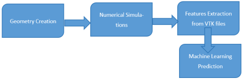
This study developed a machine-learning predictive approach for identifying dead-end pores in porous media from CFD-derived VTK data. The resulting discretized system is solved using classification models in Python. The workflow comprised four main stages which include geometry construction, numerical simulation, feature extraction from VTK files, and machine-learning classification. A flowchart for the computational approach adopted for this study is shown in
Figure 2.
Figure 2. Methodology Workflow.
2.1. Governing Equations
Fluid flow in incompressible Newtonian systems is governed by the Navier-Stokes equations, which express conservation of momentum and mass. For the present steady-state flow analysis, the governing equation may be written as , while mass conservation is enforced through the incompressibility condition (Akanji and Matthai, 2009; Ayuba et al., 2021). No-slip boundary conditions were imposed at all fluid-solid interfaces, and gravitational effects were incorporated through the pressure relation (Akanji and Matthai, 2009). The simplified form of the governing equation used in the simulation follows the computational approach described by Adeleye and Akanji (2022).
2.2. Geometric Model Construction
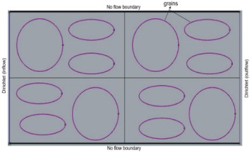
Figure 3. 2D channel with CAD model grains.
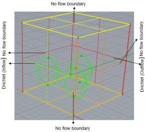
Figure 4. 3D channel CAD model with packed spheres.
Two-dimensional and three-dimensional porous geometries were created in a Computer-Aided Design (CAD) software environment to represent a range of channel-like and packed-structure configurations. The models were built using Non-Uniform Rational B-Spline (NURBS) curves and surface representations to preserve geometric fidelity and smooth curvature while maintaining computational practicality. Absolute, relative, and angular tolerances were applied throughout the modeling processes to minimize numerical distortion and preserve key structural details. Examples of the constructed geometries are shown in
Figures 3 and 4.
2.3. Numerical Simulation
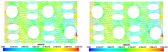
Figure 5. Velocity field simulation results of Stokes and Navier-Stokes equations for a 2D channel subjected to a pressure difference of 0.1 Pa.
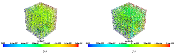
Figure 6. Velocity field simulation results of Stokes and Navier-Stokes equations for a 3D channel subjected to a pressure difference of 0.1 Pa.
The CAD-generated geometries were discretized through meshing and then subjected to fluid-flow simulation under prescribed inlet and outlet boundary conditions. Simulations were carried out in the CSMP++ platform, where physical properties and flow parameters were defined through the interrelations subclass. The solver computed the corresponding velocity and pressure fields for both Stokes and Navier-Stokes flow regimes. After the completion of the numerical runs, the generated results were post-processed to obtain pressure and velocity fields, which were then exported in VTK format for further analysis. Representative velocity-field results for the 2D and 3D channel models are shown in
Figures 5 and 6, respectively, illustrating the differences between the Navier-Stokes flow regimes under a pressure difference of 0.1 Pa.
2.4. Feature Extraction and Dataset Preparation
The simulation outputs produced a dataset of 222,810 pore-scale data points containing spatial coordinates (X, Y, Z), resultant pressure, inlet pressure, and velocity. The target labels were converted into a binary classification problem, where 0 represented non-dead-end pores and 1 represented dead-end pores. Because the dataset exhibited moderate class imbalance, class weighing was used during model training to reduce bias toward the majority class. For model development, the final predictors were X, Y, Z, and resultant pressure, as these variables captured the spatial and hydrodynamic characteristics most relevant to classification.
2.5. Machine Learning Framework
A Random Forest classifier was selected as the machine-learning framework for this study. This is because of its robustness, ability to model nonlinear relationships, and low sensitivity to feature scaling. The dataset was split into training and testing subsets using an 80/20 stratified split to preserve class proportions. In addition, a stratified subset of 20,000 points was used for visualization to reduce computational cost while retaining the original class structure. The model performance was evaluated using accuracy, precision, recall, ROC-AUC, and the confusion matrix. Three-dimensional scatter plots were also generated to assess the spatial distribution of active and dead-end pores and to support physical interpretation of the predictions.
3. Result and Discussions
3.1. Model Performance Evaluation
A Random Forest Classifier (n=100 trees) was trained on 80% of the data and evaluated on a held out 20% testing set (44,562 samples). The model performed strongly in distinguishing active pores from dead-end pores as shown by the summary metrics in
Table 1.
Table 1. Performance Metrics of the Random Forest Classifier.
Metric | Score | Interpretation |
Accuracy Score | 0.9820 | The overall probability of correct classification for any given pore. |
Precision Score (Dead-End) | 0.9768 | Of all pores predicted as dead ends, 97.68% were effectively stagnant. |
Recall Score (Dead-End) | 0.9619 | The model successfully identified 96.19% of the total dead-end volume. |
ROC-AUC Score | 0.9985 | Indicates near perfect separability between the two classes. |
3.2. Model Performance
The classifier achieved an accuracy of 98.20%, indicating a high overall rate of correct classification. For the dead-end pore class, the precision score of 0.9768 shows that most predicted dead-end pores were truly stagnant regions, while the recall score of 0.9619 indicates that the model successfully identified most of the actual dead-end pores in the test set. The ROC-AUC score of 0.9985 further confirms excellent separability between the two classes and demonstrates robust predictive performance.
The high recall of 96.19% is of particularly important in pore-scale modeling studies because missing dead-end pores can lead to underestimation of stagnant zones, solute storage, and transport resistance. In practical terms, this could affect prediction in enhanced oil recovery (EOR) and contaminant transport modeling. This is because these regions act as sinks for diffusion dominated transport or storage for residual fluids. The ROC-AUC score of 0.9985 suggests that the model is highly reliable across varying rock geometries and is not overly dependent on a single cutoff value.
3.3. Confusion Matrix Analysis
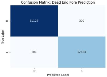
The confusion matrix provides a more detailed view of the classifier’s behaviour on unseen data. The model correctly identified 12,634 dead-end pores as true positives and 31,127 active pores as true negatives, showing strong discrimination between stagnant and conductive regions. The model produced 501 false negatives, representing dead-end pores that were missed and misclassified as active. The number of misclassifications was low. In addition, there were only 300 false positives where active pores were incorrectly labeled as dead ends.
The low false-positive rate is especially useful because it means the model rarely overestimates the volume of stagnant fluid in the porous medium. The slightly higher number of false negatives suggests that some low-velocity transition regions were labeled as active, which is reasonable for a binary classifier operating near the boundary between classes. Overall, the confusion matrix confirms that the model is both accurate and balanced in its predictions. The confusion matrix for this study is shown in
Figure 7.
Figure 7. Confusion Matrix.
3.4. Spatial Distribution of Predictions
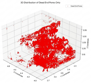
Figure 8. A 3D Distribution of Dead-End Pores.
Figure 8 shows the 3D representation of only dead-end pores. The red dots (dead-end) represent pores where the fluid velocity is stagnant (dead-ends). As shown in the plot, these tend to cluster in specific regions, likely corresponding to tighter rock formations in the pore network. The visualization clearly shows how dead-end pores are distributed relative to the main flow paths. This spatial clustering is what the machine learning model was detecting during training.
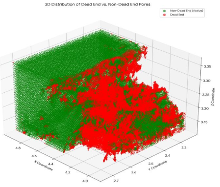
The 3D visualization shown in
Figure 9 provides a volumetric reconstruction of the porous medium, offering a direct visual comparison between the two flow regimes identified by the model. The pores visualized in green represent the active (non-dead end) regions. These elements form the continuous, conductive backbone of the rock sample. As observed in the plot, the green regions are interconnected and span the majority of the domain, illustrating the primary channels through which fluid flows under the applied pressure gradient. Their dominance in the visualization reflects the high porosity and connectivity of the rock.
The pores highlighted in bold red represent the dead-end pores. Unlike the active pores, these are not randomly scattered throughout the rock. Instead, they appear as dense, localized clusters or pockets. These red zones effectively visualize the dead-end pores of the pore network regions where the fluid is physically trapped or stagnant.
The clear spatial separation between the green (flowing) and red (stagnant) regions confirms that the machine learning model has successfully captured the physical heterogeneity of the rock. It demonstrates that dead-end pores are structural features tied to specific coordinates in the rock matrix, rather than random occurrences. The visualization validates that the model is not just predicting values, but is accurately reconstructing the internal topology of the porous medium.
Figure 9. A 3D distribution of both Active pores and Dead-End Pores.
3.5. Error Pattern
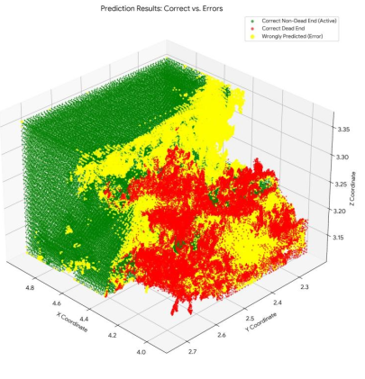
The 3D plot in
Figure 10 serves as a diagnostic tool to see exactly where the model succeeds and where it struggles within the rock structure. The majority region of the plot is dominated by green (active) and red (dead-end) points. These represent the areas where the machine learning model’s prediction perfectly matched the ground truth simulation. The clear separation between the green flow channels and the red stagnant clusters confirms that the model has successfully learned the internal geometry of the porous medium. The Yellow markers highlight the specific pores where the model made a mistake (either missing a dead end or raising a false alarm).
The most immediate observation is how few yellow dots there are compared to the red and green ones. This visual sparsity directly corresponds to the high accuracy score (approximately 98%), confirming that errors are rare events rather than systemic failures. Physically, these yellow error points are not scattered randomly. They tend to appear at the interfaces which are the thin boundary lines where a red cluster meets a green flow channel. In these transition zones, the fluid velocity is likely very low but not quite zero, making it difficult for a binary model to make a clear "yes/no" decision.
Figure 10. A 3D Distribution of Active pores, Dead-End Pores and Wrongly Predicted Pores.
4. Conclusion
This study demonstrated that a Random Forest algorithm can effectively predict dead-end pores from VTK-derived velocity-field data in porous media. Through the use of spatial coordinates and pressure-related features, the model achieved an accuracy of 98.20%, a precision of 97.68% for dead-end pores, a recall of 96.19%, and a ROC-AUC of 0.9985, indicating strong and reliable classification performance.
The spatial visualizations further confirmed that the predicted dead-end pores were clustered in physically meaningful stagnant regions rather than distributed randomly across the pore space. This shows that the model successfully captured the structural heterogeneity of the porous medium and distinguished between conductive flow channels and low-velocity dead-end zones.
The overall results show that machine-learning methods can provide an efficient and objective alternative to manual post-processing for dead-end pore identification. The proposed approach offers a scalable workflow for pore-scale flow characterization and has potential applications in enhanced oil recovery, contaminant transport, and digital rock physics.
Abbreviations
CAD | Computer-Aided Design |
CFD | Computational Fluid Dynamics |
CNN | Convolutional Neural Network |
CSMP | Complex Systems Modelling |
CT | Computed Tomography |
GNN | Graph Neural Network |
LBM | Lattice Boltzmann Method |
NURBS | Non-Uniform Rational B-Spline |
PINN | Physics Informed Neural Network |
ROCAUC | Receiver Operating Characteristic - Area Under the Curve |
VTK | Visualization Toolkit |
Author Contributions
Ibrahim Ayuba: Conceptualization, Data curation, Methodology, Project administration, Software, Validation, Writing – original draft
Yusuf Shuro Gamaliel: Formal Analysis, Investigation, Methodology, Software, Visualization, Writing – original draft
Ephraim Ojoajogu Enemali: Data curation, Formal Analysis, Validation, Visualization, Writing – review & editing
Roy Zwalatha Milton: Conceptualization, Project administration, Writing – review & editing
Abdulsalam Abdukarim: Formal Analysis, Funding acquisition, Investigation, Resources, Supervision, Writing – review & editing
Conflicts of Interest
The authors declare that they have no known competing financial interests or personal relationships that could have appeared to influence the work reported in this paper.
References
| [1] |
Bijeljic, B., Mostaghimi, P., & Blunt, M. J. (2013). Insights into non-Fickian solute transport in carbonates. Water Resources Research, 49(5), 2714-2728.
|
| [2] |
Valvatne, P. H., & Blunt, M. J. (2004). Predictive pore-scale modeling of two-phase flow in mixed wet media. Water Resources Research, 40(7).
|
| [3] |
Andrew, M., Bijeljic, B., & Blunt, M. J. (2014). Pore-scale imaging of trapped carbon dioxide in sandstones and carbonates. International Journal of Greenhouse Gas Control, 22, 1-14.
|
| [4] |
Soulaine, C., Gjetvaj, F., & Tchelepi, H. A. (2021). Pore-scale description of multiphase flow in porous media: Revisiting the role of the wetting phase. Transport in Porous Media, 140(1), 1-26.
|
| [5] |
Zhang, R., Wang, L., & Chen, S. (2019). Lattice Boltzmann method for multiphase flows: Theory and applications. Advances in Applied Mechanics, 52, 1-87.
|
| [6] |
Mostaghimi, P., Blunt, M. J., & Bijeljic, B. (2013). Computations of absolute permeability on micro-CT images. Mathematical Geosciences, 45(1), 103-125.
|
| [7] |
Santos, J. E., et al. (2020). Machine learning for fluid flow in porous media: A review and new perspectives. Advances in Water Resources, 142, 103656.
|
| [8] |
Sudakov, O., Burnaev, E., & Koroteev, D. (2021). Driving digital rock towards machine learning: Predicting permeability with convolutional neural networks. Computational Geosciences, 25, 955-972.
|
| [9] |
Loucks, R., Reed, R., Ruppel, S., & Hammes, U. (2012). Spectrum of pore types and networks in mudrocks and a descriptive classification for matrix-related mudrock pores. AAPG Bulletin, 96(6), 1071 - 1098.
https://doi.org/10.1306/08171111061
|
| [10] |
Ayuba, I., Akanji, L. T., Gomes, J. L., & Falade, G. K. (2021). Investigation of drift phenomena at the pore scale during flow and transport in porous media. Mathematics, 9, Article 2509.
https://doi.org/10.3390/math9192509
|
| [11] |
Mosser, L., Dubrule, O., & Blunt, M. (2017). Reconstruction of three-dimensional porous media using generative adversarial neural networks. Physical Review E, 96, 043309.
https://doi.org/10.1103/physRevE.96.043309
|
| [12] |
Telvari, S., Sayyafzadeh, M., Siavashi, J., Sharifi, M. (2021). Prediction of two-phase flow properties for digital sandstone using 3D convolutional neural networks. Advances in Water Resources, 176, 104442.
https://doi.org/10.1016/j.advwatres.2023.104442
|
| [13] |
Alqahtani, N., Niu, Y., Wang, Y., Chung, T., Lanetc, Z., Zhuravljov, A., Armstrong, R., & Mostaghimi, P. (2022). Super-Resolved Segmentation of X-ray Images of Carbonate Rocks Using Deep Learning. Transport in Porous Media, 142, 497-525.
https://doi.org/10.1007/s11242-022-01781-9
|
| [14] |
Santos, J., Chang, B., Gigliotti, A., Yin, Y., Song, W., Podanovic, M., Kang, Q., Lubbers, N., & Viswanathan, H. (2022). A Dataset of 3D Structural and Simulated Transport Properties of Complex Porous Media. Scientific Data 9(579).
https://doi.org/10.1038/s41597-022-01664-0
|
| [15] |
Li, H., Zhang, Y., Wang, D., et al. (2024). Gradient information enhanced image segmentation and automatic parameter extraction for digital rock physics. Water Resources Research, 60(9), e2023WR036869.
https://doi.org/10.1029/2023WR036869
|
Cite This Article
-
APA Style
Ayuba, I., Abdulkarim, A., Gamaliel, Y. S., Enemali, E. O., Milton, R. Z. (2026). Machine Learning Prediction of Dead-end Pores from VTK Based Velocity Fields in Porous Media. International Journal of Oil, Gas and Coal Engineering, 14(3), 61-69. https://doi.org/10.11648/j.ogce.20261403.12
 Copy
|
Copy
|
 Download
ACS Style
Ayuba, I.; Abdulkarim, A.; Gamaliel, Y. S.; Enemali, E. O.; Milton, R. Z. Machine Learning Prediction of Dead-end Pores from VTK Based Velocity Fields in Porous Media. Int. J. Oil Gas Coal Eng. 2026, 14(3), 61-69. doi: 10.11648/j.ogce.20261403.12
Copy
|
Download
AMA Style
Ayuba I, Abdulkarim A, Gamaliel YS, Enemali EO, Milton RZ. Machine Learning Prediction of Dead-end Pores from VTK Based Velocity Fields in Porous Media. Int J Oil Gas Coal Eng. 2026;14(3):61-69. doi: 10.11648/j.ogce.20261403.12
Copy
|
Download
-
@article{10.11648/j.ogce.20261403.12,
  author = {Ibrahim Ayuba and Abdulsalam Abdulkarim and Yusuf Shuro Gamaliel and Ephraim Ojoajogu Enemali and Roy Zwalatha Milton},
  title = {Machine Learning Prediction of Dead-end Pores from VTK Based Velocity Fields in Porous Media},
  journal = {International Journal of Oil, Gas and Coal Engineering},
  volume = {14},
  number = {3},
  pages = {61-69},
  doi = {10.11648/j.ogce.20261403.12},
  url = {https://doi.org/10.11648/j.ogce.20261403.12},
  eprint = {https://article.sciencepublishinggroup.com/pdf/10.11648.j.ogce.20261403.12},
  abstract = {Dead-end pores are important microstructural features in porous media because they strongly influence flow efficiency, transport behaviour, and solute retention. However, their identification remains challenging due to geometric complexity and the limitations of conventional post-processing methods. In this study, we developed a machine-learning framework for the automated prediction of dead-end pores from pore-scale velocity-field data obtained through numerical fluid-flow simulations. Two-dimensional and three-dimensional porous geometries were constructed using CAD tools and simulated under Stokes and Navier-Stokes flow regimes using the CSMP platform. The resulting pressure and velocity fields were exported in Visualization Toolkit (VTK) format, and spatial as well as hydrodynamic features were extracted for analysis. A supervised classification approach based on a Random Forest model was trained on 222,810 pore-scale data points, using spatial coordinates and pressure as predictor variables. Dead-end pores were defined as stagnant regions weakly connected to the main flow pathways and labelled accordingly. Model performance was evaluated using accuracy, precision, recall, and ROC-AUC, along with three-dimensional visualizations for physical validation. The proposed model achieved an accuracy of 98.20%, a recall of 96.19% for dead-end pore identification, and a ROC-AUC score of 0.9985, indicating excellent predictive performance and robustness. These results show that machine learning can reliably distinguish active flow channels from stagnant dead-end regions directly from velocity-field data without explicit connectivity analysis. The approach offers a scalable and objective tool for pore-scale characterization with potential applications in enhanced oil recovery, contaminant transport, and digital rock physics.},
 year = {2026}
}
Copy
|
Download
-
TY  - JOUR
T1  - Machine Learning Prediction of Dead-end Pores from VTK Based Velocity Fields in Porous Media
AU  - Ibrahim Ayuba
AU  - Abdulsalam Abdulkarim
AU  - Yusuf Shuro Gamaliel
AU  - Ephraim Ojoajogu Enemali
AU  - Roy Zwalatha Milton
Y1  - 2026/06/30
PY  - 2026
N1  - https://doi.org/10.11648/j.ogce.20261403.12
DO  - 10.11648/j.ogce.20261403.12
T2  - International Journal of Oil, Gas and Coal Engineering
JF  - International Journal of Oil, Gas and Coal Engineering
JO  - International Journal of Oil, Gas and Coal Engineering
SP  - 61
EP  - 69
PB  - Science Publishing Group
SN  - 2376-7677
UR  - https://doi.org/10.11648/j.ogce.20261403.12
AB  - Dead-end pores are important microstructural features in porous media because they strongly influence flow efficiency, transport behaviour, and solute retention. However, their identification remains challenging due to geometric complexity and the limitations of conventional post-processing methods. In this study, we developed a machine-learning framework for the automated prediction of dead-end pores from pore-scale velocity-field data obtained through numerical fluid-flow simulations. Two-dimensional and three-dimensional porous geometries were constructed using CAD tools and simulated under Stokes and Navier-Stokes flow regimes using the CSMP platform. The resulting pressure and velocity fields were exported in Visualization Toolkit (VTK) format, and spatial as well as hydrodynamic features were extracted for analysis. A supervised classification approach based on a Random Forest model was trained on 222,810 pore-scale data points, using spatial coordinates and pressure as predictor variables. Dead-end pores were defined as stagnant regions weakly connected to the main flow pathways and labelled accordingly. Model performance was evaluated using accuracy, precision, recall, and ROC-AUC, along with three-dimensional visualizations for physical validation. The proposed model achieved an accuracy of 98.20%, a recall of 96.19% for dead-end pore identification, and a ROC-AUC score of 0.9985, indicating excellent predictive performance and robustness. These results show that machine learning can reliably distinguish active flow channels from stagnant dead-end regions directly from velocity-field data without explicit connectivity analysis. The approach offers a scalable and objective tool for pore-scale characterization with potential applications in enhanced oil recovery, contaminant transport, and digital rock physics.
VL  - 14
IS  - 3
ER  -
Copy
|
Download