Overview on Spectral Analysis Techniques for Gamma Ray Spectrometry

Masayuki Imaizumi

doi:doi:10.11648/j.ns.20240901.12

Review Article |

| Peer-Reviewed

Overview on Spectral Analysis Techniques for Gamma Ray Spectrometry

Masayuki Imaizumi^*

Published in Nuclear Science (Volume 9, Issue 1)

Received: 26 March 2024 Accepted: 17 April 2024 Published: 10 May 2024

Views: Downloads:

Download PDF

Share This Article

Twitter
Linked In
Facebook

Abstract

Gamma-ray spectrometry (GRS) is an exploration technology that distinguishes itself from other non-contact sensing technologies because it provides information from 30 to 50 cm below the ground. This technology has evolved through three significant turning points in mapping output. The first turning point, in the 1960s-1970s, was the transition from U concentration maps to weathered zoning maps utilizing K or eTh. The second turning point, occurring from the 1980s to 1990s, was marked by the application of radionuclide mapping to assess radioactive contamination. A third turning point, in the early 2000s, was the development of soil maps for precision agriculture, supported by the free statistics software R. This paper reviews advances in gamma-ray spectrometry spectral analysis since 2000. Traditionally, the gamma-ray spectrum is depicted as a two-dimensional graph with energy on the horizontal axis and counts on the vertical axis. The NASVD and MNF methods, developed around 2000, necessitate a reevaluation of this concept. By conducting principal component analysis of the gamma-ray spectrum in hyperspace, these techniques have unveiled new spectra, such as ground and sky spectra, and have facilitated the removal of noise components from the gamma-ray spectrum. Naturally occurring gamma-ray spectra typically exhibit energies ranging from 0.04 to 3 MeV. Observations from fusion reactors measure energies up to 20 MeV for diagnostics of nuclear plasma. These spectra may yield valuable insights when applied to innovative statistical analysis techniques. A comprehensive spectral analysis method developed in the early 2000s has demonstrated the potential to extract a variety of information beyond window nuclides, previously unexplored. The regression coefficient plots from the PLSR regression model have revealed novel spectral images. This model is set to influence future research on GRS by expanding the number of objectives and covariates. The innovative calibration method for full-spectrum analysis, which assesses different concentration areas, has proven that calibration is achievable even in the absence of a calibration pad. It is expected to become a formidable approach for spectrum analysis in the upcoming period.

Published in	Nuclear Science (Volume 9, Issue 1)
DOI	10.11648/j.ns.20240901.12
Page(s)	8-29
Creative Commons	This is an Open Access article, distributed under the terms of the Creative Commons Attribution 4.0 International License (http://creativecommons.org/licenses/by/4.0/), which permits unrestricted use, distribution and reproduction in any medium or format, provided the original work is properly cited.
Copyright	Copyright © The Author(s), 2024. Published by Science Publishing Group

Keywords

Hyperspace, Principal Component Analysis, Regression Analysis, Partial Least Squares Regression Analysis, Regression Coefficients Plots, Full-Spectral Analysis

1. Introduction

Gamma-ray spectrometry (GRS) is an exploration technology that distinguishes itself from other non-contact sensing technologies because it can provide information from 30 to 50 cm below the surface. GRS has a long-standing history since the 1940s, when total gamma-ray measurements were utilized for uranium exploration. The nomenclature for gamma-ray spectrometry varies depending on the platform of the detector acquiring the gamma-ray spectrum: airborne (airborne gamma-ray spectrometry survey, AGRS), where measurement equipment is mounted on an aircraft or helicopter; carborne, which involves mounting a measuring device on a vehicle; manborne, where an individual carries a detector and measures at a fixed point or while moving. More recently, measurements using unmanned aerial vehicles and drones have been added to AGRS (e.g.,

[1]

). Carborne now includes field tractor measurements (e.g.,

[2, 3]

). Additionally, there are the gamma-ray logging method, which involves measurements in a borehole, and the Seaborn method, which involves placing a measuring device on the seabed or towing it along the seabed

[4]

From the 1940s to the 1950s, GRS could not discriminate radionuclides, but since the mid-1960s, the need to monitor the effects of nuclear tests and advances in computer technology have made field measurement of potassium (K), uranium (U), and thorium (Th) possible. The International Atomic Energy Agency (IAEA) began studies in the 1970s to standardize gamma-ray spectrometry. This effort led to the publication of the first standard technical guide in 1991

[5]

. In 2003, the IAEA released a second guideline that incorporated the theory of gamma-ray spectrometry, expanding its application to environmental surveys beyond traditional geological survey purposes

[4]

. This development finalized the technical framework

[6]

The gamma-ray spectrum measured by the NaI detector is a two-dimensional chart that depicts the relationship between channels and gamma-ray intensity, segmenting energy from 0 to 3 MeV into more than 256 channels. Since there are only three nuclides—potassium (K), uranium (U), and thorium (Th)—with photoelectric peaks that are identifiable in the spectrum, nuclide concentration analysis is performed using an analysis method known as the window method (See Section 3.2). This method focuses on a specific window delineated around the energy peak of each of the three nuclides

[4]

. Therefore, it is important to note that the data used are solely the total counts from 0 to 3 MeV and the counts within the nuclide-specific window. In essence, a significant portion of the measured data is not used in the window method analysis.

GRS has evolved into a mature measurement method since IAEA

[4]

equipped with sophisticated instruments and standardized analytical methodologies

[6]

. Currently, innovative detectors with enhanced sensitivity have enabled the mapping of subtle variations in potassium (K), thorium (Th), and uranium (U) concentrations with improved accuracy and higher resolution. However, gamma-ray data are influenced not only by the original lithology but also by overlapping data from regolith and soil. Consequently, it is not possible to uniquely determine the primary lithology or delineate the secondary alteration history based solely on the concentrations of K, Th, and U elements. One of the ongoing challenges is the development of technologies that effectively utilize concentration data of U, Th, and K measured by gamma-ray spectroscopy. Another challenge is the development of new spectral analysis methods, which may involve leveraging previously unused data.

This technology has evolved through three significant turning points in mapping output. The first, which spanned the 1960s to 1970s, involved transitioning from U concentration maps to weathered zoning maps using potassium (K) or equivalent thorium (eTh). The second turning point, occurring from the 1980s to 1990s, was marked by the application of radionuclide mapping to assess radioactive contamination. The third turning point, in the early 2000s, was the development of soil maps for precision agriculture, which were supported by freely available statistics software.

In addition to gamma-ray spectrometry, methods for detecting uranium deposits include soil radon gas surveys, which measure alpha particles emitted by radon gas in the soil. Suran

[7]

investigated which radiological exploration method was most instrumental in discovering the 164 uranium (U) deposits in the Czech Republic between 1946 and 1990. He determined that the soil radon (Rn) gas survey was the most effective, accounting for 44% of the discoveries, while AGRS and carborne surveys were less effective, contributing to only 3% and 9% of discoveries, respectively. This result is not surprising, considering that uranium deposits are generally deemed commercially viable if they have a grade of 0.1% (1000 ppm) or higher

[8]

. For example, a 3σ confidence level U anomaly detected by an 8.4 Liter NaI (Tl) detector at an altitude of 80 m can identify a concentration of 4860 ppm U within a 4 m diameter, but only 9 ppm U at a 100 m diameter

[4]

. Thus, Suran’s findings indicate that mapping uranium anomalies with AGRS presents challenges in directly pinpointing uranium mines.

The reason why γ-ray spectrometry, especially AGRS, had regained attention in the field of exploration is that γ-ray spectrometry found not only U and Th deposits but also many metals deposits in the altered zone defined as the high K and low Th/K ratio (e.g.,

[9]

). This is the first turning point in the development of technology for using gamma-ray spectrometry. This tipping point occurred due to the understanding of radionuclide behavior in hydrothermal and alteration/weathering processes. Since this turning point, AGRS has been accepted as a geological survey technique for mapping wide-area radionuclide concentration zones, rather than as a technique for exploring the location of anomalous radiation spots.

The second turning point of the GRS was triggered by the application of the AGRS to the exploration of two artificial radioactive materials; one was the fragment exploration of the crash of the Soviet nuclear satellite COSMOS 954 in January 1978 in northwestern Canada. The other is the mapping of radioactively contaminated areas from the 1986 Soviet Union Chernobyl nuclear accident

[10]

. Since then, GRS has established its role as a tool for preparing for nuclear emergencies and mapping the environment. AGRS has also been used to assess the causes of indoor radon contamination

[10, 11]

In the 2000s, the concept of precision agriculture was introduced into the field of agriculture. Until the 1980s, the mainstream approach in agriculture was to increase yield by using large amounts of fertilizers and pesticides, but this led to various issues, including the decline of soil fertility and environmental concerns. Consequently, the concept of precision agriculture, which aims to maintain yield with a minimal and sustainable input of fertilizers and pesticides, has gained global recognition. Precision agriculture is defined as a series of agricultural management methods that follow the Plan-Do-Check-Act cycle, such as deliberate monitoring of the state of farmland and farm products, careful control of soil conditions, and planning the next year’s cropping based on these results

[12]

. Supporting this approach is the development of new sensor technologies for understanding soil characteristics and crop growth. Non-contact soil analysis methods for soil moisture, pH, electrical conductivity, etc., have been developed, but non-contact soil analysis methods for soil texture, total carbon, total nitrogen, nitrate nitrogen, etc., have not yet been established

[12]

McBratney et al. (2003)

[13]

discussed mapping techniques in a comprehensive review of digital soil mapping techniques. They highlighted that the primary role of AGRS is as an alteration zone mapping tool, but its potential as a soil moisture measurement tool

[14]

, utilizing the attenuation effect of gamma rays, is also promising. IAEA (2010)

[15]

did not mention the agricultural applications of gamma-ray spectrometry in their reports. Therefore, it can be stated that at least before 2010, there was limited recognition among researchers that gamma-ray spectrometry could serve as a tool for mapping soil characteristics, such as soil texture.

However, since the late 1990s, some studies have begun to explore the use of gamma-ray signals, particularly potassium (K) and thorium (Th), as sensors for pH meters and plant-available potassium (e.g.,

[16, 17]

). In the 2000s, the application of gamma-ray spectrometry as a soil texture mapping tool was proposed as a novel sensor technique for precision agriculture (e.g.,

[18]

). Since 2010, research employing GRS as a soil property sensor has advanced rapidly. Notably, promising studies include those on soil classification (e.g.,

[19, 20]

), peatland mapping tools (e.g.,

[21, 22]

), soil texture (e.g.,

[23, 24]

), plant-available potassium (e.g.,

[25, 26]

), and pH

[27]

, among others.

When employing γ-ray spectrometry as a tool in soil science, it is crucial to perform regression analysis to investigate the relationship between soil characteristics and radionuclide concentrations, going beyond the traditional γ-ray analysis techniques. Regression analysis includes not only simple linear regression but also more sophisticated methods that utilize a range of explanatory covariates, such as geostatistical models and machine learning algorithms. As explanatory variables, it is possible to use not only topographic maps (digital elevation models) but also categorical variables like soil and geological maps. The practicality of such analyses has been made possible by the widespread availability of free statistical software since 2000, with the programming language R playing a pivotal role in this development. The first version of R was released to the general public in 2000, and a distinctive feature of R is its library of over 13,200 packages, which are available for free and cater to specialized fields. Many R textbooks have been published (e.g.

[28]

). These packages include tools for principal component analysis and partial least squares methods for spectral analysis. The third wave of innovation in GRS appears to have begun around 2000, driven by the demand for new sensor technologies in precision agriculture and the enhancement of gamma-ray analysis through the support of the aforementioned free software.

Despite advancements as recent as those following IAEA (2003)

[4]

, comprehensive summaries of these developments remain scarce. This paper reviews advances in γ-ray spectrometric analysis since 2000. The regression analysis of soil texture will be reported on another occasion. Sections 2 and 3 delve into the radioactive decay process and the methods of γ-ray spectral analysis. Specifically, a method for projecting a γ-ray spectrum into a higher-dimensional space and reducing noise through principal component analysis—a widely-used chemometric technique—is discussed. With respect to the implementation of principal component analysis of γ-ray spectra, an example using R’s chemoSpec package is provided. Section 4 demonstrates the application of the partial least squares (PLS) method, another chemometric technique, to γ-ray spectra and details the implementation of PLS using R’s pls package. The paper concludes with a summary in section 5.

2. Radioactive Decay Processes

2.1. Radioactivity

Radioactivity is a phenomenon in which an atomic nucleus with an unstable balance of protons and neutrons transforms into a stable nucleus by emitting elementary particles such as alpha particles (α-radiation), beta particles (β-particles), and gamma photons (γ-rays) over time. Elements that exhibit this behavior are termed radionuclides. The rate of atomic decay per unit time is statistically proportional to the existing number of atoms, irrespective of other physical states, and is expressed by the following equation

[4]

N_{t} = N_{0} e^{- λt}

(1)

where, N_t is the number of atoms existing after the lapse of time t (s). N₀ is the number of atoms existing at time t = 0. λ is the decay constant (s^-1), and e is the base of the natural logarithm.

Alpha rays are helium (He) nuclei composed of 2 protons and 2 neutrons. They lose energy by colliding with other particles. The air absorption range of alpha rays is several centimeters, and for rocks, it is virtually negligible. Beta rays are electrons produced when neutrons are converted into protons. The air absorption range is about 1 meter, and for rocks, it is negligible. Conversely, gamma rays are electromagnetic waves of excess energy emitted when an unstable excited nucleus transitions to a new stable state. Unlike alpha and beta rays, they have no mass. When γ-rays pass through matter, they interact with the electrons and nuclei of the atoms in the material through phenomena such as the photoelectric effect, Compton scattering, and pair production

[4]

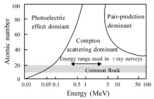
The photoelectric effect is a predominant interaction with low-energy γ-rays, where all γ-ray energies are absorbed through collisions with electrons. Compton scattering is a medium-energy dominant interaction that results in the loss of some gamma-ray energy upon collision with electrons and subsequent scattering at an angle. Electron-positron pair production occurs at energy levels exceeding 1.02 MeV. At this threshold, the incident γ-ray energy is completely absorbed, resulting in the generation of an electron-positron pair.

Download: Download full-size image

Figure 1. Attenuation effects across energy ranges and typical interactions of gamma-rays with materials of varying atomic numbers (Modified from

[29]

In the practical context of soil science, Compton scattering predominates. Gamma radiation from soil is primarily attenuated by water, soil, and organic matter

[30]

(see Figure 1).

2.2. Interaction Between Neutrons and Matter

Other nuclear transformations include spontaneous fission and electron capture. Spontaneous fission is a process where atomic nuclei spontaneously split. The likelihood of spontaneous fission is elevated in transuranic elements with an atomic number (Z) of 93 or greater, such as curium (²⁴⁴Cm) and plutonium (²⁴⁰Pu). This process emits fast neutrons, which are neutral particles within the atomic nucleus. Neutrons are inherently unstable and undergo beta decay. Their lifespan is approximately 1000 seconds, and the maximum energy of the emitted beta particle is 780 keV

[29]

Neutrons may be classified according to their kinetic energy (En) as follows

[29]

Cold neutrons: En < 0.025 eV

Thermal neutrons: En ~ 0.025 eV

Slow neutrons: 1 eV < En < 300 eV

Intermediate neutrons: 300 eV < En < 1 MeV

Fast neutrons: 1 MeV < En < 20 MeV.

Neutrons that are emitted from the nucleus during spontaneous fission, artificial fission, and fusion are classified as fast neutrons.

The interactions between γ-rays and matter, and between neutrons and matter, are markedly different. γ-rays primarily interact with orbital electrons due to the Coulomb repulsive force acting between charged particles, resulting in ionization. Conversely, neutrons, having no charge, interact directly with nuclei as they are unaffected by the Coulomb force. The interaction of neutrons with matter is broadly categorized into scattering and absorption.

Scattering is further subdivided into elastic and inelastic scattering. During elastic scattering, the kinetic energy of the colliding particles is conserved. In inelastic scattering, a portion of the kinetic energy is transferred to the nucleus as excitation energy. Nuclei excited to a level capable of emitting gamma rays revert to the ground state by emitting gamma rays. If γ-rays cannot be emitted, processes such as alpha-ray emission and nuclear fission occur, leading to a more stable state

[29]

During the absorption process, neutrons are captured by the nucleus. Subsequently, the atomic nucleus enters an excited state with additional energy due to the kinetic energy of the captured neutrons. This excess energy is expended to emit other particles and gamma rays. When emission occurs as gamma rays, it is termed “radiative capture”. The radiative capture reaction, where neutrons are incorporated into the nucleus, does not alter the atomic number but increases the mass number by one

[29]

The nuclear reaction equation for elastic scattering is expressed as X(n, n)X, where X represents the target/residual nucleus, and n denotes the neutron. The reaction (n, n) is referred to as the “(n, n) reaction”. Given that the mass of a proton is nearly identical to that of a neutron, the hydrogen target nucleus acquires the maximum energy—equivalent to one proton—while the neutron loses the most energy

[29]

In inelastic scattering accompanied by nuclear reactions, there are numerous possible reactions, and the specific reaction that occurs is dependent not only on the type of target nucleus but also on the neutron’s energy. The primary reactions for low-energy neutrons are neutron capture and elastic scattering. For thermal neutrons, the predominant reaction is neutron capture. In the neutron capture reaction, the nuclei that absorb the neutrons and become excited subsequently emit only gamma rays with an energy of 2.2 MeV. This reaction is known as the (n, γ) reaction. When light nuclei such as Li and Be absorb neutrons, they emit alpha particles. This reaction is termed the (n, α) reaction

[29]

2.3. Environmental Radionuclides

2.3.1. Natural Radionuclides

Radionuclides in the environment originate from three sources: cosmic rays, natural processes, and human activities. There are 22 nuclides of cosmic ray origin, such as ³H and ¹⁴C, but they do not interfere with γ-ray spectrometry since they are low-energy β-ray emitters.

Natural radionuclides were formed during the Earth’s creation and concentrated in the crust, yet most have transformed into stable nuclides after 4.5 billion years. Presently, there are 17 nuclides with a half-life exceeding 700 million years. Among the existing nuclides, only ⁴⁰K, ²³⁸U, and ²³²Th exhibit significant radioactivity and are analyzed using γ-ray spectrometry. Gamma rays are also emitted from ²¹⁴Pb and ²²⁸Ac, but due to their low counting rate, they are not the target nuclides for gamma ray analysis described below. 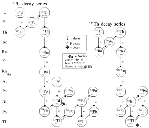⁴⁰K constitutes 0.012% of potassium (K), with 83.3% being a β-ray emitting nuclide, and 10.7% decaying to ⁴⁰Ar through EC (electron capture), emitting a 1.46 MeV γ-ray in the process.²³⁸U and ²³²Th decay to produce daughter nuclides, which further undergo radioactive decay, forming a decay chain (Figure 2). The decay from ²³⁸U to stable ²⁰⁶Pb primarily occurs through α decay, although β decay and γ decay also occur. Only²¹⁴Bi and ²⁰⁸Tl are the nuclides that emit γ-rays targeted in γ-ray spectrometry.

Download: Download full-size image

Figure 2. Radioactive decay series of ²³⁸U and²³²Th. The 238U decay series was adapted from Wikipedia. The 232Th decay series was adapted from Wikimedia Commons.

Since the half-life of each parent nuclide in a series is significantly longer than that of its daughter nuclides, the radioactivity of each nuclide in the series approaches a steady state in secular equilibrium, which is equivalent to that of the parent nuclide in a closed system. In secular equilibrium, the radioactivity of all nuclides in the series is equal, so the concentration of a nuclide at one stage of the decay chain can be estimated from the concentration of all daughter nuclides.

When one or more decay products in the decay chain are completely or partially removed or added to the system, the decay chain enters a state of disequilibrium. Since ⁴⁰K does not create a decay chain, it is unaffected by the non-equilibrium problem. Theoretically, it takes 40 years for the ²³²Th series to establish secular equilibrium, and more than 1.5 million years for the ²³⁸U series

[31]

. In the ²³²Th series, a non-equilibrium state rarely occurs due to the low mobility of daughter nuclides. However, in the ²³⁸U series, non-equilibrium states are more likely due to selective leaching of decay products (e.g., ²²⁶Ra), diffusion of ²²²Rn gas from soil, and dissolution of ²²⁶Ra in groundwater

[9]

Since ⁴⁰K exists in a fixed ratio to the non-radioactive K isotope, K (%) can be directly analyzed from ⁴⁰K γ-rays of GRS. The U concentration of GRS is estimated from ²¹⁴Bi γ rays of the daughter nuclide of ²³⁸U. Thus, the uranium concentration by GRS is an indirectly estimated concentration. Therefore, the uranium concentration (ppm) analyzed by GRS is indicated as eU (equivalent Uranium) concentration to distinguish it from the U concentration determined by chemical analysis. Similarly, since the Th concentration is estimated from ²⁰⁸Tl γ rays of the daughter nuclide of ²³²Th, the Th concentration (ppm) is expressed as the eTh concentration

[4]

2.3.2. Artificial Radionuclides

Artificial radionuclides are those that do not occur naturally but are synthesized through various processes. They include nuclides of fission products generated in nuclear experiments and nuclear reactors, nuclides activated within nuclear reactors, reaction nuclides produced in fusion reactors, and those resulting from man-made satellite accidents.

A fission reaction is a process where unstable nuclides of heavy nuclei split, producing two or more lighter elements. This splitting releases an average of 2-3 fast neutrons. These neutrons are then reabsorbed by another ²³⁵U atom, leading to a fission chain reaction that initiates subsequent fission reactions. Fission products are nuclides created by fission and those resulting from the radioactive decay of fission fragments. Even with the same ²³⁵U, the substances produced by nuclear fission vary with each event. There are hundreds of different substances that can be produced by nuclear fission.

The Fukushima Daiichi Nuclear Power Station accident dispersed fission product nuclides into the environment as fallout

[32]

. Among the fallout nuclides, those with a high production rate (yield) and relatively long half-life include ¹³⁷Cs, ¹⁰³Ru, ¹⁴⁰Ba, and others. ¹³⁴Cs is not a fission product; it is formed by neutron activation of the stable fission product ¹³³Cs in the reactor. Consequently, the amount of ¹³⁴Cs varies depending on the type of fuel rods and the reactor’s operational duration. This variation means that the ¹³⁴Cs/¹³⁷Cs ratio serves as an indicator to identify the reactor source. Additionally, since ¹³⁴Cs is not present in the fallout from nuclear tests, the presence or absence of ¹³⁴Cs can distinguish between fallout from nuclear tests and that from nuclear power plant accidents

[33]

Fusion involves merging light nuclei, such as hydrogen in a plasma state, into heavier nuclei like helium, a process that emits neutrons. In 1985, it was proposed to conduct fusion research for peaceful purposes through international collaboration. This research is ongoing under the ITER program, currently in its second phase, aiming to establish scientific and technological feasibility. One fusion reactor design under consideration utilizes high-temperature plasma to magnetically confine deuterium (D) and tritium (T) in a tokamak configuration. In the D-T fusion reaction, radionuclides such as helium nuclei (alpha particles), neutrons, tritium, and activated dust emitting γ-rays are produced

[34]

3. Gamma Ray Spectral Analysis Method

3.1. Gamma Ray Measurement Mechanism and Detector

The energy of gamma rays can be measured by scintillation detectors and Ge semiconductor detectors. The scintillation detector consists of a scintillator (crystal), a photomultiplier tube, and peripheral devices such as a pulse height analyzer. The emitted photon ejects an electron from the negative electrode of the photomultiplier tube. When this electron collides with the anode, a voltage pulse with a negative amplitude proportional to the energy of the incident photon is generated

[4]

. The energy spectrum is the result of analyzing the amplitude of the voltage pulse with a pulse height analyzer across 256 to 1,024 multiple channels (ch).

Scintillation detectors contain various substances. Table 1 presents the parameters of typical scintillation and semiconductor detectors.

Table 1. Parameters of Typical Scintillation and Semiconductor Detectors.

	Detector type	Resolution 662keV (%)	Density (g/cc)	Light Yield (Photons/keV)	Decay time (ns)	Dead time (s)	Remarks
Scintilla-tor detector	NaI (Tl)	7	3.7	38	250	10^-7s order	Deliquescent
	BGO	14	7.13	9	300
	CsI	10	4.53	56	1000	10^-9s order	Weak Deliquescent
	LaBr₃ (ce)	2.8-4.0	5.29	63	16		Deliquescent
	CeBr₃	4	5.2		18-20
Semi -conductor	CdTe	2.0-2.5					Room temperature
Semi -conductor	HPGE	0.2 (1.3 keV)	5.35	N/A	N/A		Liquid N cooling

Download: Download full-size image

Figure 3. Gamma-Ray Spectrum of Soil in Tsukuba City, Japan: (a) Spectrum of Ge(Li) Semiconductor Detector, and (b) Spectrum of NaI Detector. The spectra at the bottom of the figure are the standard spectra for each nuclide according to Hendriks et al.

[37]

: 40K (solid line), 238U (dotted line), and 232Th (one-dot chain line).

NaI crystal detectors are primarily utilized in field surveys. NaI crystals are transparent, have a high density (3.7 g/cm³), and can be produced in large volumes. The dead time is on the order of 10^-7 seconds. However, even with a NaI detector with a resolution of 7 to 10%, the peak shape of the nuclide broadens, causing the peaks of adjacent energies to overlap. Consequently, only ²¹⁴Bi, ⁴⁰K, and ²⁰⁸Tl of natural radionuclides can be unequivocally identified as individual nuclides (Figure 3). Since the NaI detector is hygroscopic, it becomes fragile after many years of use. CsI crystals, on the other hand, are not hygroscopic and are more robust than NaI crystals. Their density is 4.51 g/cm³ and the dead time is on the order of 10^-9seconds. However, they are inferior to NaI crystals in terms of resolution, emission yield (luminescence), and decay time. BGO (Bi₄Ge₃O₁₂) crystals have a high density (7.13 g/cm³), are not hygroscopic, and are more efficient even for high-energy γ-rays, but their resolution is inferior to that of NaI and CsI crystals.

Lanthanum bromide, LaBr₃(Ce), discovered in 2000

[35]

, exhibits superiority over NaI in terms of density (5.3 g/cm³), resolution (2.8-4.0%), decay time, and emission yields (Table 1). The primary concerns with LaBr₃(Ce) are its hygroscopic nature and the radioactivity of ¹³⁸La present within the crystals. Such radioactivity elevates the background noise and compromises detectability to some extent. Consequently, a cerium bromide, CeBr₃, detector was developed

[36]

. This detector possesses a density of 5.2 g/cm³ and a resolution of 4%, with performance marginally less effective than LaBr₃(Ce). Nonetheless, CeBr₃ demonstrates approximately an order of magnitude greater detection sensitivity for higher-energy nuclides, such as ⁴⁰K at 1462 keV and ²⁰⁸Tl at 2614 keV. Owing to its non-hygroscopic properties, CeBr₃ proves to be superior to LaBr₃(Ce) for use in field surveys.

None of the scintillation detectors mentioned above can achieve the resolution (0.2%) of the HPGe semiconductor detector (Table 1: Figure 3). A spectrum peak of HPGe is detected as a very sharp spectral line. However, due to the requirement for cooling the detector with liquid nitrogen during measurement, its use has been limited to laboratory measurements. Recently, the development of the pulse tube refrigerator, which allows for outdoor use, has facilitated the use of HPGe in the field. Most recently, it has become possible to use a lightweight Cadmium zinc telluride (CZT) semiconductor detector at ambient temperature. Although its resolution (2-2.5%) is not as high as that of HPGe, its portability is another advantage. Martin et al.

[36]

and Marques et al.

[1]

demonstrated that the CZT detector could be used for unmanned investigations with drones.

In fusion plasma, neutrons and gamma rays, which are unaffected by the magnetic field, can be detected by dedicated diagnostic equipment. Neutron emission spectrometry (NES) and gamma-ray spectrometry (GRS) are used as principal methods for studying fast ions

[38]

. Neutron spectrometry is used to diagnose the suprathermal component of fuel ions. Gamma-ray spectrometry is used to diagnose fusion-produced alpha particles and high-energy ions. The severe environment of a fusion plasma reactor makes it difficult to detect gamma rays, thus a dedicated diagnostic system is required. In the JET (Joint European Torus) tokamak reactor, collimated gamma rays are recorded by Ge semiconductor detectors and scintillators (NaI, BGO, LaBr3, etc.) located in a well-shielded bunker

[38]

3.2. γ Ray Spectrum

There is a certain relationship between the channel of the pulse height analyzer and the γ-ray energy. Therefore, the channel axis can be converted to the energy axis by energy calibration using known energy nuclides in the spectrum. The natural origin gamma-ray spectrum usually displays energies ranging from 0.04 to 3 MeV

[4]

. Fusion reactor observations measure energies up to 20 MeV

[38]

. Here, we will focus on the natural gamma-ray spectrum.

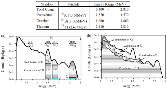
As previously mentioned, the γ-ray spectrum of the NaI detector can detect γ-ray nuclides such as 40K and the daughter nuclides of the Th and U series. Displayed below the NaI spectrum in Figure 3 are the separate γ-ray spectra for 40K, U, and Th

[37]

. The spectrum measured in situ is a composite in which the spectra of the three nuclides overlap with the background.

The ⁴⁰K spectrum shows the energy distribution of single-energy gamma rays. The peak near 1.46 MeV is the peak of the photoelectric effect. The total energy Eγ of γ-rays is transferred to electrons in the photoelectric effect, so the energy distribution forms a linear peak located at Eγ. This is called a photoelectric peak or a total absorption peak. The actual peak shape is a spreading mountain shape due to statistical fluctuations. A gentle slope continues on the low energy side (left side) of the peak. This part is called the Compton continuum. The Compton continuum is the part where gamma rays interact with the source, the air between the source and the detector, and the detector, partially losing energy of γ-ray due to Compton scattering at various angles. One photoelectric peak and Compton scattering are paired. The spectrum of ²³⁸U has peaks at 1.12 MeV and 609 keV of ²¹⁴Bi in addition to the photoelectric peak of ²¹⁴Bi at 1.76 MeV. The ²³²Th spectrum has peaks at 2.1 MeV and 969-911 keV of ²⁰⁸Tl in addition to the photoelectric peak of 2.62 MeV of ²⁰⁸Tl. However, when these peaks overlap, the only peaks that can be discriminated are the three spectra of ⁴⁰K (1.46 MeV), ²³⁸U (²¹⁴Bi, 1.76 MeV), and ²³²Th (²⁰⁸Tl, 2.62 MeV).

Gamma-ray spectral analysis typically involves Total Count (TC), window analysis (WA), or full spectrum analysis (FSA) within the energy range of 0.4 to 3 MeV (Figure 4). Most gamma-ray spectrometry analyses are TC and WA. In WA, the count of the range of interest (ROI) (referred to as the energy window) centered on the photoelectric peaks of ⁴⁰K, ²¹⁴Bi, and ²⁰⁸Tl is analyzed. If ¹³⁷Cs (662keV) fallout is present, ¹³⁷Cs can also be detected by monitoring a 100 keV wide window centered on the photoelectric peaks of these nuclides. Since the peak shape follows a normal distribution, the ROIs for WA are defined by the full width at half maximum (FWHM) of the peak. The IAEA

[4]

guideline ROIs are depicted in Figure 4. The counts for each window include background (BG) and Compton scattering (CS) counts, as well as counts proportional to the radionuclide concentration. Thus, the BG and CS counts must be subtracted from the counts in each window to obtain counts solely proportional to the radionuclide concentration.

Electron pair generation occurs within sub-nanosecond timescales following the incidence of gamma rays. Therefore, when one of the two photons generated by pair production escapes from the detector, an energy of E - 511 keV is observed as a single escape peak in the spectrum of the Ge semiconductor detector. If both photons escape, an energy of E - 1022 keV is observed as a double escape peak

[29]

Since window analysis (WA) focuses only on the areas of interest for ⁴⁰K, ²³⁸U, and ²³²Th, the gamma-ray count for each window is two orders of magnitude lower than the total count (TC), potentially leading to inaccuracies in estimated concentrations for short-term measurements. Moreover, the energy resolution of the NaI detector at 583 keV (²⁰⁸Tl) and 609 keV (²¹⁴Bi) complicates the analysis of trace amounts of 662 keV (¹³⁷Cs). Full spectrum analysis (FSA) was developed to address this issue. As FSA utilizes the entire spectral range, it requires significantly fewer statistics to achieve the necessary accuracy, thus reducing the time needed for stable measurements (e.g.,

[37, 39]

). However, Mahmood et al.

[40]

applied both the window and full-spectral methods to predict soil texture and other parameters in the same field. They concluded that both methods could establish a relationship between radionuclide data and soil quality with as much accuracy as possible.

Download: Download full-size image

Figure 4. The energy range of the Total Counts and windows

[4]

and schematic diagram of the window method (a) and full spectrum method (b) (Modified from

[41]

). (a) The SC method obtains the photoelectric peak count by subtracting the Compton scattering count of the nuclide at higher energy from the ROI count (n). The SC for estimating the Compton scattering count from ²³²Th is α. The SC of the scattering count from ²³²Th in the potassium window is βand the SC from ²³⁸U is γ. For NaI detectors, some of the potassium peaks also affect the number of windows for uranium and thorium on the higher energy side. This effect is treated with inverse stripping coefficients a, b, g, but is usually ignored. (b) In the full spectrum method, the measured spectrum (N) is the standard spectrum (Sk) (the ⁴⁰K, ²³⁸U and ²³²Th spectra at the bottom of Figure 3) multiplied by the radionuclide concentration (Ck) of the individual radionuclides. Details are given in Section 3.5.3.

The use of gamma-ray detection as a diagnostic tool for tokamak fusion plasmas has evolved over the decades. Historically, gamma-ray spectroscopic analysis for nuclear reactions in plasma has been proposed as a complementary tool to neutron flux measurements to assess the rate at which energy-generating reactions occur. Gamma-ray emission in fusion plasma results from the reactions of fuel nuclei or rapidly moving charged particles with plasma impurities

[38]

. Gamma-ray measurements in fusion plasmas can be used to diagnose nuclear reaction rates and the densities of nuclear reaction products (e.g.,

[38]

). Table 2 provides a list of nuclear reactions identified by the JET

[38]

Table 2. List of nuclear reactions emitting γ-rays identified at JET

[38]

Reaction	Q [MeV]	Emin [MeV]	Reaction	Q [MeV]	Emin [MeV]
Protons			Tritons
D(p,γ)³He	5.5	0.05	D(t,γ)⁵He	16.63	0.02
T(p,γ)⁴He	19.81	0.05	⁹Be(t,nγ)¹¹B	9.56	0.5
⁹Be(p,p'γ)⁹Be	-2.43	3	³He ions
⁹Be(p,γ)¹⁰Be	6.59	0.3	D(³He,γ)⁵Li	16.38	0.1
⁹Be(p,αγ)⁶Li	2.125	2.5	⁹Be(³He,nγ)¹¹C	7.56	0.9
¹²C(p,p'γ)¹²C	-4.44, -7.65	5, 8	⁹Be(3He, dγ)¹¹B	10.32	0.9
Deuterons			⁹Be(3He,dγ)¹⁰B	1.09	0.9
⁹Be(d,pγ)¹⁰Be	4.59	0.5	¹²C(³He, pγ)¹⁴N	4.78	1.3
⁹Be(d,nγ)¹⁰B	4.36	0.5	Alphas
¹²C(d,pγ)¹³C	2.72	0.9	⁹Be(⁴He, nγ)¹²C	5.7	1.9

3.3. Influential of Terrain Features for Gamma Ray Measurement

GRS estimates nuclide concentrations based on the assumption that the detector detects radiation from a flat 180° (2π steradians) solid angle terrain. When measurements are taken with a portable detector placed in concave terrain, radiation from a solid angle region of 2π steradians or more is incident on the detector, leading to an overestimation of the radiation distribution. Conversely, when measurements are taken with a device placed on a bank or at the edge of recessed terrain, radiation from a solid angle region less than 2π steradians is incident on the detector, resulting in an underestimation

[42]

. Since gamma rays can travel through the air for hundreds of meters, GRS is also influenced by distant terrain. For instance, when GRS measurements are conducted along a survey line from coastal waters to 10-meter-high granodiorite cliffs far away, the dose rate may increase due to the cliff’s influence

[42]

. These phenomena must be considered, especially when measurements are required in spaces surrounded by valleys and slopes

[42]

For AGRS measurements on flat terrain, gamma rays from a diameter area approximately twice the altitude (h) account for 66% of the total count. In valleys, the total count may increase by 100% because the area is influenced by the slopes of both valleys. On ridges, since this area is reduced, the total count may decrease by 10% to 30%

[10]

. Minty and Brodie

[43]

propose a three-dimensional (3D) inverse analysis method to correct for the topographical effects on AGRS. This method takes into account the detector’s directional sensitivity, movement velocity, and 3D topographical data within the detector’s field of view to inversely analyze the ground element concentration into a regular grid.

3.4. Metrology of Gamma Ray Spectrometry

3.4.1. Portable Device for Man-Borne

A 0.1 to 0.35 L NaI crystal is typically used for a portable gamma-ray spectrometer. The detector is placed directly on the ground surface or held at a constant height (e.g., waist position) during measurement to minimize the influence of ground surface irregularities and local changes in radionuclide distribution. It is also feasible to conduct surveys while walking at a consistent pace. When the detector is placed on the soil surface, it measures gamma rays from a diameter of approximately 2 meters and a depth of 25 centimeters

[4]

. When the detector is placed on an exposed rock surface, it measures gamma rays from a radius of about 1 meter and a depth of 15 centimeters

[42]

. The measurement duration is typically several hundred seconds. The error in the measured value using the 0.35 L NaI detector is 10% for 2 minutes on ground with high radionuclide concentration and for 6 minutes on ground with low concentration

[4]

. The survey line intervals for reconnaissance and detailed surveys are set at 50 to 250 meters and 5 to 10 meters, respectively. The measurement point spacing is set to 5 meters in both cases

[4]

3.4.2. Device for Car-Borne and Agricultural Tractors Survey

Car-borne is a method for filling the gap between man-borne and AGRS

[4]

. Typically, the car-borne detector uses a 4 to 8 L NaI detector, which is smaller than the AGRS detector. As with the AGRS system, the car-borne system standardly features GPS navigation with detailed road maps displayed. Additionally, some are equipped with an alarm system that audibly notifies the operator of the target position

[4]

. The movement speed of the car-borne system is 1/5 to 1/10 that of the AGRS. Measurements are usually taken at intervals of several tens of seconds

[15]

. The measurement area of the NaI detector in the car-borne system has a radius of 6 meters. When moving at 4 km/h, the measured value for 30 seconds represents the integrated count over an extension of 33.3 meters.

Geological mapping by car-borne systems should utilize unpaved, off-road survey data. Even off-road data can obscure the original geological conditions, as the roads may be significantly contaminated with substances used in road construction

[4]

. Therefore, the primary application of car-borne systems is addressing environmental issues, such as the search for lost radiation sources and fallout mapping. Since these target nuclides are anthropogenic radionuclides that exceed natural background levels, the development of paved road networks is actually advantageous for car-borne investigations. In fact, the KURAMA car-borne system, equipped with a CsI scintillation detector developed by the Kyoto University Research Reactor Institute, was deployed for the distribution survey of radioactive materials released from the Fukushima Daiichi Nuclear Power Station accident

[44]

Since 2000, tractor-mounted Proximal Mobile Gamma Spectrometry (PMGS) has been applied to soil mapping for precision agriculture. In PMGS, the detector is fixed in front of the tractor on a shelf 30 centimeters above the surface of the earth. The measurement methods are classified into running (on-the-go) measurement and stop-and-go measurement. The detector, positioned 30 centimeters above the ground, measures soil gamma rays with a radius of approximately 2 meters and a depth of 0.3 meters. The accuracy of both measurements is almost the same (R² = 0.96)

[3]

. The detectors used for PMGS include a 1 to 2 × 4.2 L NaI detector

[3, 24, 26]

and a φ70 × 150 mm CsI detector

[45]

, among others. The running speed for the on-the-go survey is applied at 0.7 to 1.4 meters per second

[3]

, 0.83 meters per second

[26]

, and 2.8 meters per second

[45]

. The sampling time is at 1-second intervals. In the stop-and-go survey, spectra are acquired every 60 seconds

[23]

. The distance between survey lines is 6 to 27 meters, depending on the condition of the field.

3.4.3. Device for Airborne

The AGRS standard system comprises a ground measuring device and an atmospheric radon measuring device. The ground measuring device is designed for detecting γ-rays emanating from the ground surface. It is composed of two units, each containing 16.4 L NaI detectors. Each unit houses four sets of detectors, with one set featuring a 10.2 cm x 10.2 cm x 40.6 cm NaI crystal and a photomultiplier tube, encased in a heat insulating container. The atmospheric radon measuring device is mounted atop the ground measuring device. A lead plate measuring 35 x 45 x 2 cm is interposed between the two devices to attenuate gamma rays from the ground, thereby enhancing the upper detector’s sensitivity to sources above

[4]

Gamma rays emanating from the ground towards the AGRS are attenuated by atmospheric density. To correct the AGRS gamma ray measurements for ground altitude, the following data are recorded every second during the survey: GPS (with an error of approximately 5 meters), radar altimeter (with a 2% error), barometer, and thermometer

[4]

. A standard pulse height analyzer possesses a channel range of at least 256 channels (Ch). Furthermore, cosmic rays with energies exceeding 3.0 MeV may be detected in supplementary windows

[4]

AGRS measurements are typically conducted along a grid-based flight path. The spacing of flight lines for geological and environmental mapping ranges from 50 to 400 meters

[4]

. The flight altitude varies from 30 to 300 meters above ground level, and for helicopters, it is between 40 and 100 meters. Recent AGRS measurements are often taken at an altitude of approximately 120 meters

[4]

. In the 2005-2006 Tellus Aerial Geophysical Survey project in Northern Ireland conducted by the British Geological Survey, the AGRS had a survey line spacing of 200 meters, with a flight altitude of 244 meters in urban areas and 56 meters in rural areas

[46]

. For soil mapping in Australia, the AGRS utilized a measurement line spacing of 100 meters and a flight altitude of 20 meters

[27]

. In Sweden, the AGRS featured a line spacing of 200 meters with an altitude ranging from 30 to 60 meters

[47]

. The flight speed for the AGRS is approximately 50 to 60 meters per second, and for helicopters, it is 25 to 30 meters per second. The sampling interval is typically 1 second for aircraft and 0.5 seconds for helicopters.

Approximately 80% of the γ-rays detected by AGRS originate from the top 0.3m of soil within the measurement area, the radius of which is roughly four times the flight altitude

[4]

. Given a radionuclide concentration in the soil of 2% K, 2.5ppm U, and 9ppm Th, the measurement accuracy (expressed as standard deviation) of a typical AGRS is 6.3% for K, 12.3% for eU, and 13.7% for eTh

[42]

. The accuracy of the AGRS increases as the flight altitude decreases. Unmanned helicopters and drones (UAVs) are capable of measuring γ-rays from an altitude of 30 m above the ground

[36]

, making them a potentially promising tool, particularly in the field of precision agriculture

[48]

3.5. Spectrum Processing

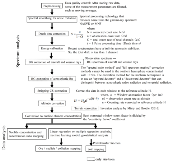
3.5.1. Data Processing Procedure

Figure 5 illustrates the data processing workflow for TC and WA. The section enclosed by the solid line in the figure represents the data processing procedure for man-portable, car-mounted, and AGRS systems. The section enclosed by the dashed line is an addition to the AGRS analysis. The common data processing procedure includes the following steps: (1) preprocessing tasks such as data verification and conversion of GPS information to a mapping coordinate system, (2) smoothing of spectra for noise reduction (using NASVD or MNF methods), (3) dead time correction, (4) energy calibration, (5) background correction for cosmic rays and aircraft, (6) correction for atmospheric Rn, (7) Compton scattering correction using the stripping method, (8) aircraft altitude correction (air attenuation correction), (9) anomaly analysis and spectral analysis, (10) conversion of radionuclide concentrations using sensitivity coefficients, (11) terrain correction, (12) regression/geostatistical analysis, (13) distribution pattern analysis, (14) thematic map creation, and (15) data storage

[2, 5, 30]

. The processing methods for steps (4), (7), and (10) differ for FSA compared to WA. As previously mentioned, gamma-ray spectrometry is a well-established technique. Therefore, the techniques introduced after the IAEA’s publications in 2003

[4]

and 2010

[15]

are limited, such as the terrain effect correction technique by Minty and Brodie

[43]

. This document will provide explanations on spectrum smoothing technology, full-spectrum analysis, and gamma-ray diagnostics for nuclear plasma, with the aim of supplementing the IAEA’s guidelines

[4]

. Data analysis from steps (12) to (14) is a new addition, primarily for the creation of soil maps. These steps will be explained in a separate paper. For more information on spectral analysis, please refer to the IAEA

[4, 5]

Download: Download full-size image

Figure 5. Flow Chart of Data Processing for TC and Window Analysis (The spectrum analysis section was developed with reference to IAEA

[5]

, Rossel et al.

[2]

, and Reinhardt and Herrmann

[30]

3.5.2. Spectrum Smoothing (Noise Reduction) Technology

The γ-ray spectrum is depicted as a two-dimensional graph, with energy (or channels) on the horizontal axis and counts on the vertical axis. However, in chemometrics, spectral analysis is conducted in a multidimensional space. To project the spectrum into this space, the spectral data is converted into a matrix. In chemometrics, analysis of the spectrum in multidimensional space is carried out using statistical methods such as principal component analysis (PCA)

[49]

. Techniques for smoothing the γ-ray spectrum and comprehensive spectrum analysis draw upon chemometric principles. For instance, if we consider the γ-ray spectrum X₁, comprising 256 channels, as “one point in a 256-dimensional space,” it can be represented by the following equation:

X_{1} = (α_{1_1}, α_{1_2}, α_{1_3}, \dots \dots, α_{1_256})

(2)

Although it is not possible to visualize a space of four or more dimensions, we can analyze the spectrum with an analogous concept in a three-dimensional space

[49]

. According to this concept, the spectrum is represented by a single point in the multidimensional space, regardless of the spectrum’s complexity. When the γ-ray spectrum of the same radioactive element as X1 varies solely in element concentration, the spectral points in the multidimensional space are plotted along the line extending from X₁ to the coordinate origin. If the spectrum’s shape alters due to the presence of different elements, the spectrum’s position will deviate from the line connecting the origin and point X₁, since Eq. (4) is no longer valid. In other words, spectra with distinct shapes will have different trajectories when viewed from the origin of multidimensional space. The spectrum’s shape is associated with the direction from the origin of the multidimensional space, while the spectrum’s intensity (element concentration) corresponds to the distance from the origin. In essence, the multidimensional space, also known as hyperspace

[49]

, is a convenient framework where changes in the spectrum can be distinctly categorized into alterations in shape and intensity.

The NASVD method (Noise Adjusted Singular Value Decomposition) and the MNF method (Maximum Noise Fraction) are techniques for smoothing the γ-ray spectrum. They eliminate noise components from the original γ-ray spectrometry data by applying principal component analysis within the γ-ray spectrum hyperspace

[4]

. The principle operates as follows: Principal component analysis breaks down the original hyperspectral data into several constituent components. The spectrum is then reconstructed using only the components that are not identified as ‘noise’. This reconstructed spectrum retains most of the original signal while significantly reducing the noise. The primary distinction between the NASVD and MNF methods lies in the normalization approach for the noise components within the spectrum. Nevertheless, both methods achieve a comparable level of noise reduction

[4]

Only PCA will be described here. The PCA model formula is written as follows

[36]

X = T P^{T} = t_{1} p_{1}^{T} + t_{2} P_{2}^{T} + t_{3} p_{3}^{T} + \dots

(3)

where, t_j is an eigen-orthogonal vector used to express X in a vector space and is referred to as a loading vector (or simply loading). A loading is a vector that can efficiently characterize the spectral plot points in multidimensional space; that is, it represents a new principal axis (principal component axis) that indicates the direction of significant variance (corresponding to eigenvalues) in the spectrum. t_j is a projected value measurable on the new axis (loading), which can be calculated by the dot product of X and p_j. The t_jis termed a score vector (or simply a score)

[50]

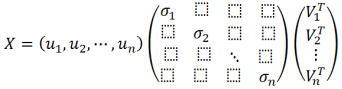
In practice, when performing principal component analysis (PCA) using statistical software on a personal computer, singular value decomposition (SVD) is employed to derive eigenvalues and eigenvectors. SVD decomposes any given matrix into two orthogonal matrices and a diagonal matrix. The singular values are the diagonal entries σ of the diagonal matrix. PCA results vary based on the scaling of variables in X; therefore, it is standard to normalize the variance of the scores for all variables to 1. Consequently, the score matrix (T) is normalized to matrix (U), and the scalar quantities of each component are consolidated into matrix (S). Assuming the loading matrix is (V) (which, despite the notation (V), is equivalent to loading (P)), the singular value decomposition is expressed as shown in Eq. (4):

X = T P^{T} = US V^{T}

(4)

U and V^T are orthogonal matrices, and S is a diagonal matrix where the explained variance from each component is on the diagonal, and all other entries are zero. The equation for isolating only the first principal component is as follows:

(5)

The singular values σ are selected to satisfy the following conditions:

σ₁≥σ₂≥・・・・≥σ_n

The eigenvectors of (U) represent the spectra of the principal components. When the observed spectrum is transformed into the orthogonal spectral components as per Eq. (4), it is decomposed into scores and loadings of 6 to 8 components. Each component is ranked according to its contribution to the observed spectrum. Meaningful signals that correlate across channels are prioritized in the first principal component. Conversely, random noise tends to be distributed evenly across all channels and is not interrelated. Consequently, random noise is relegated to the lower-order components. By reconstructing the spectrum using only the significant signal components from the adjusted set of spectral components, it is possible to generate a spectrum devoid of noise

[4]

PCA transforms the multidimensional spatial structure (i.e., direction from the origin) of the original spectrum through principal component transformation. Additionally, the position indicating the concentration (i.e., the distance from the origin) becomes indeterminate. Consequently, the inherent meaning within the spectrum may seem obscured. However, despite the altered coordinate system and the quantitative change in the spectrum’s shape, the integrity of the data is maintained. The essence of the spectrum remains unchanged; it is merely the representation that differs

[49]

. Thus, the principal components derived from PCA are synthetic variables created by transforming the original measurement data, necessitating careful interpretation of what each principal component axis represents

[50]

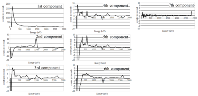
Figure 6 illustrates an example of NASVD (Noise Adjusted Singular Value Decomposition) applied to the aerial gamma-ray spectrum

[6]

. Graphs 1 to 7 display the seven components resulting from the NASVD decomposition. The seventh component is regarded as random noise. The first six components are utilized for reconstructing a noise-reduced spectrum. The first component is presumed to reflect the average spectrum of the entire dataset. The 2nd to 6th components influence the shape of the measured spectrum, each exerting distinct effects

[6]

. For instance, the second and third components exhibit a peak near 1400 keV for potassium (K) and both a positive and negative peak near 2600 keV for thorium (Th). The sixth component shows a negative peak for K and a positive peak for Th. These peaks are believed to correspond to the ground concentrations of potassium (K), uranium (U), and thorium (Th). Conversely, in the 4th and 5th components, K and Th manifest as negative peaks, while only at 1700 keV does uranium (U) present a positive peak. These components also align with the pronounced photoelectric peaks of radon (Rn) at 352 keV, 609 keV, and 1120 keV, suggesting that this source is atmospheric radon, proximal to the detector. Hence, the U peak at 1700 keV is interpreted as indicative of the influence of atmospheric Rn

[6]

Download: Download full-size image

Figure 6. Example of NASVD Decomposition in Airborne Gamma-Ray Spectrometry. The first seven components of the NASVD decomposition (Fortin et al.

[6]

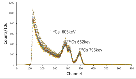
The final part of this section provides an example of principal component analysis (PCA) of gamma-ray spectra, conducted using the chemoSpec package

[52]

in R. The ten gamma-ray spectra, displayed in Figure 7, were recorded by Imaizumi et al

[51]

from paddy soils contaminated by the Fukushima Daiichi nuclear event. These spectra were obtained through a man-borne survey utilizing a 3 x 3-inch NaI detector with 1024 channels. The measurement duration for each spectrum was ten seconds. The three prominent peaks in the Figure 7 observed between channels 350 and 500 correspond to the photoelectric absorption peaks of ¹³⁴Cs at 605 keV, ¹³⁷Cs at 662 keV, and ¹³⁴Cs at 796 keV.

Download: Download full-size image

Figure 7. 10 gamma ray spectra measured by Imaizumi et al

[51]

on paddy field soil in Iitate Village, Fukushima Prefecture in August 2011.

Download: Download full-size image

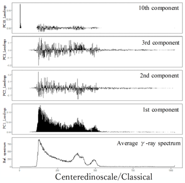
Figure 8. Loading plot of the gamma-ray spectrum from Iitate village’s rice field. The figures, from the bottom to the top, represent the average γ-ray spectrum, the 1st, 2nd, 3rd, and 10th principal components of the loading plots.

To perform PCA on gamma-ray spectra with the chemoSpec package, the spectrum CSV file is first converted into a spectrum object. This conversion is carried out using the matrix2SpectraObject function (note that this is distinct from the standard R read.csv function). Once transformed into a spectral object, PCA analysis can be conducted using the c_pcaSpectra function. As the aim here is not to compare the spectra, normalization of the spectra is not performed. The summary function and scree plot reveal that the spectrum of 1024 channels was decomposed into 10 principal components. The first principal component accounts for 80% of the variance. It was demonstrated that 95% of the gamma-ray spectrum variance could be explained by the first to seventh principal components (not shown here). Figure 8 is loading plots of gamma-ray spectrum of Iitate village rice field. Figures from the bottom to the top show loading plots of the average γ-ray spectrum and the 1st, 2nd, 3rd, and 10th principal components, respectively.

PCA simply linearly transforms the data and rotates it within a multidimensional space. Therefore, if the principal component axis, which has been rotated by an angle Θ, is rotated by -Θ, it can be reverted to its original orientation. All software that performs PCA can calculate rotation matrices. In R’s principal component analysis, rotation data is stored in the $rotation slot. Thus, to reconstruct the spectrum using principal components while excluding the 10th principal component, identified as noise, the scores from the 1st to 9th principal components are multiplied by the transposed matrix of the rotation matrix. Consequently, the original spectrum, excluding the 10th principal component, can be retrieved.

3.5.3. Processing of Compton Scattering Counts for Window Analysis

The count rate c/s (counts per second) per unit concentration (1% K, 1 ppm U, and 1 ppm Th) is referred to as the sensitivity coefficient

[4]

. The concentrations of ⁴⁰K (C_K), ²³⁸U (C_U), and ²³²Th (C_Th) are determined by dividing the photoelectric peak count of each nuclide by the sensitivity coefficient (S) established during calibration. However, the U window counts include Compton scattered counts from Th-series nuclides in addition to the 1.76 MeV photoelectric peak count. Similarly, the K window counts encompass Compton scattered counts for both Th-series and U-series nuclides, along with the 1.46 MeV photoelectric peak count. Consequently, it is necessary to correct for Compton scattering to accurately determine the photoelectric peak counts for U and K window counts. This correction can be performed using either the Kobel method or the Stripping Coefficient (SC) method. The Kobel method is employed when a distinct photoelectric peak is present and is primarily used for spectral analysis with Ge semiconductors and NaI detectors in laboratory settings. In contrast, the SC method is a straightforward semi-quantitative approach utilized in field applications and is commonly employed in window analysis (WA).

The SC method is predicated on the pairing of a photoelectric peak with Compton scattering, and it posits that the Compton scattering count can be approximated by a specific ratio of the photoelectric peak count. This implies that the window count (n) consists of the photoelectric peak count (np) that defines the window and the Compton scattering count (photoelectric peak count n_pH × SC) of the high-energy nuclide (n_pH). The Compton scattering count is corrected by subtracting (n_pH × SC) from (n). The SC for estimating the Compton scattering count from Th in the uranium window count is α. The SC for the scattering count from Th in the potassium window is β, and the SC from U is γ (Figure 4a). Consequently, the concentrations of ⁴⁰K, ²³⁸U and²³²Th (C_K, C_U, and C_Th) are expressed as follows:

The concentration of potassium (C_K) is calculated as:

C_{k} = (n_{K} - β n_{Th} - γ (n_{U} - α n_{Th})) / S_{K}

(6)

The concentration of uranium (C_U) is determined by:

C_{U} = (n_{U} - α n_{Th}) / S_{U}

(7)

And the concentration of thorium (C_Th) is:

C_{Th} = n_{Th} / S_{Th}

(8)

where n_K, n_U, and n_Th are the net counts in the K, U, and Th windows, respectively, corrected for the detector and cosmic ray background. S_K, S_U, and S_Th are the sensitivity coefficients for K, U, and Th, respectively.

In the case of the NaI detector, its inadequate resolution means that part of the potassium peak count also influences the uranium and thorium window counts on the high energy side. Strictly speaking, this effect should be addressed with inverse stripping coefficients a, b, and g, but it is typically disregarded

[10]

. Since the interaction of gamma rays with each detector varies even for identical concentrations of radioactive elements, the stripping coefficient must be calibrated using a standard radiation source for each specific detector

[4]

3.5.4. FULL-Spectrum Analysis

In this technique, the (almost) full energy spectrum is considered, and the measured spectrum (N) is described as the sum of the standard spectra (S_k) multiplied by the activity concentrations (C_k) for the individual radionuclides, plus a background spectrum (B)

[39]

N (i) = \sum_{k = 1}^{4} C_{k} S_{k} (i) + B (i)

(9)

where N(i) are the counts in channel (i), Ck are the concentrations of element (k), Sk(i) are the associated counts to the fundamental spectrum of element (k) in channel (i), and B(i) are the counts in channel (i) due to the intrinsic background. The index k stands for ⁴⁰K, ²³²Th, ²³⁸U, and ¹³⁷Cs. A standard spectrum represents the response of the detector in a given geometry to an activity concentration of 1 Bq/kg for a given radionuclide. ⁴⁰K is given in percent weight, while equivalent uranium (eU) and equivalent thorium (eTh) are given in ppm

[39]

If, for a particular geometry, the standard spectra S_k and the background spectrum B(i) are known, the measured spectrum N(i) can be analyzed with the standard spectra by a procedure that identifies the optimal C_k values and minimizes χ² as per the following equation:

χ^{2} = \frac{1}{n - 5} \sum_{i = 1}^{n} {[N (i) - \sum_{k = 1}^{4} C_{k} S_{K} (i) - B (i)]}^{2} / N (i)

(10)

where N(i) is considered as Poisson distributed and n is the number of channels in the spectrum utilized in the analysis

[39]

The standard spectra for the individual radionuclides, S, are determined from measurements of samples with well-known activity concentrations. Because the samples will contain trace elements of more than one radionuclide, their combined concentrations constitute the activity concentration matrix, N. The calibration spectra, C, are measured for each calibration sample. The standard spectra S are then derived from the matrix equation [N]=[C]×[S] and are calculated by inverting the concentration matrix M in [S]=[C]⁻¹×[N]. The FSA calibration method also generates a unique background B that can be compared with a spectrum acquired with the detector inside a thick lead shielding

[39]

The FAS calibration method by Caciolli et al.

[39]

utilizes a site characterized by one of the natural radionuclides in the field, as opposed to the conventional concrete pad method. Given the near impossibility of selecting sites with only a single nuclide, calibration is conducted at eight sites featuring unbalanced nuclide concentrations in the field. The criteria for site selection are as follows:

A relatively uniform distribution of radionuclides in secular equilibrium with their decay products.

A flat area without steps, sufficiently large to be considered an infinite source (maximum radius 10 m).

An undisturbed area, ensuring a relatively constant vertical distribution of ¹³⁷Cs.

A relatively uniform soil moisture content and vegetation coverage.

The concentrations of the four nuclides at each site were analyzed via gamma-ray spectrometry in the laboratory, with samples collected from 5 to 12 random locations within a 10 m radius around the detector. Utilizing this calibration data, the concentration error in the verification test was found to be 5% for ⁴⁰K, 7% for ²³²Th, and 15% for ²³⁸U

[39]

3.5.5. Gamma-Ray Diagnostics for Nuclear Plasma

The D-T fusion reactions may be direct (one-step) reactions such as

[38]

;

d+t→γ+⁵He(11)

The energies of the gamma rays are determined by the simultaneous requirement of energy and momentum conservation during the reactions. For the generic reaction

[38]

M₁+M₂→M₃+γ(12)

E_γ=E₀+Q(1–Q/(2M₃))(1+2(v_CM/c)Cos(θ))(13)

where, M is the rest energies of the masses. Q is the energy of the mass residuals of a substance; Q = M₁ + M₂-M₃. E₀ is the sum of the center of mass kinetic energies of the reactants; E₀ = E₁ + E₂. v_CM is the speed of the center of mass of the reactants relative to the observer. θ is the angle of the gamma ray in the coordinate system of the observer relative to the direction of the center of mass motion of the initial reactants

[38]

Evidence of fusion is observed by detecting 5.5 MeV gamma rays from the reaction D (p, γ)³He. The energies of the observed gamma rays will thus be in an approximately symmetric distribution with the centroid of the distribution at:

E_γ=Q(1–Q/(2M₃))+E_G(14)

Download: Download full-size image

Figure 9. Gamma-ray spectrum measured during JET discharge with ICRF heating in deuterium JET plasma. The spectrum calculated by means of the program GAMMOD (dashed line)

[38]

Figure 9 shows the peak of 5.5 MeV gamma rays emitted from the capture reaction D (p, γ)³He and the simulation spectrum by the program GAMMOD. 5.5 MeV gamma rays confirm that protons were generated in the plasma. The figure not only displays the gamma peak of the capture reaction but also the gamma peak of the ¹²C (d, pγ) ¹³C reaction. According to GAMMOD, the effective tail temperatures of hydrogen minority ions and deuterium are 0.20 ± 0.05 MeV and 0.1 MeV, respectively

[16]

4. Partial Least Squares Regression Analysis

Section 3.5.2 describes the chemometric method whereby the γ-ray spectrum is projected onto a hyperspace and noise is reduced through principal component analysis. Within chemometrics, both principal component analysis and the partial least squares method are employed as standard techniques. For noise reduction, the spectrum X was decomposed into principal components, the noise component was isolated, and the spectrum was reconstructed excluding the noise component.

The standard principal component regression (PCR) approach analyzes the principal components of X and isolates those that encapsulate the correlated variables. However, as the principal components of X lack the information of Y, the outcomes of the PCR may not always yield significant insights. Conversely, the partial least squares method (PLS) decomposes X into components that incorporate information about Y, facilitating a more informed regression analysis.

Partial least squares regression (PLSR) is a modeling technique developed in the field of econometrics by Wold et al.

[53]

. It is particularly effective when dealing with a large number of explanatory variables, such as the spectral data from a machine analyzer, or when there is multicollinearity among the explanatory variables. Rossel et al.

[2]

were the first to apply PLSR to gamma-ray spectrometry for predicting soil texture. This document presents application examples of gamma-ray spectrometry using PLSR by Rossel et al.

[2]

and Kassim et al.

[26]

. Additionally, it outlines the procedure for implementing PLSR using the ‘pls’ package in R. For an in-depth understanding of the mathematical principles of PLSR, please refer to the manual

[54]

Rossel et al.

[2]

utilized the chemometrics software ParLeS v2.1 for spectral preprocessing, PCA analysis, PLSR modeling, and prediction. The analysis results are displayed in the spectra of the correlation coefficient for each of the 256 channels. Clay content spectra at soil depths of 1-15 cm exhibited a strong positive correlation at 1,420 keV: K and 2,700 keV: Th. The correlation between the measured and predicted values was (R² = 0.77). Conversely, the spectra of sand content at soil depths of 15-50 cm demonstrated a weak negative correlation at 1,420 keV and 2,700 keV. The correlation between the measured and predicted values was (R² = 0.79).

Download: Download full-size image

Figure 10. Scatter plot of laboratory-measured available potassium (K_a) (mg 100 g−1) and predicted K_a by the third-order polynomial function (3DPF) (a) and partial least squares regression (PLSR) analysis and regression coefficients plots (c)

[26]

Kassim et al.

[26]

applied two regression analysis methods to predict the potassium (K_a) available to plants in soil: (1) ⁴⁰K by window analysis of γ-ray spectra and K_a analyzed in the laboratory. Nonlinear polynomial regression of (2) Partial least squares regression (PLSR) of full spectrum and laboratory analysis K. R’s “prospectr” package

[54]

was used for preprocessing of the gamma-ray spectrum. The R “pls” package

[53]

was used to build the PLSR regression model. Figure 10 shows the comparative results of the nonlinear polynomial regression model and the PLSR regression model. In the nonlinear polynomial regression model, the cubic polynomial model showed the highest (R² = 0.69). The optimal model for PLSR showed (R² = 0.85). The largest positive peak of PLSR’s Regression coefficients plots indicates that the 1,420 keV (⁴⁰K) band contributes most to the PLSR prediction. The second largest positive correlation peak is associated with the ²³²Th band at 2,700 keV. They considered why the PLSR prediction (R²) was higher than the nonlinear polynomials; (⁴⁰K) was affected by the non-uniform pH of the soil. On the other hand, PLSR did not use (⁴⁰K) as a predictor, so the effect of pH was small.

PLSR can be executed using the ‘pls’ package. This section outlines the PLSR implementation method as described in the manual by Mevik and Wehrens

[53]

. The dataset used is the ‘gasoline’ dataset included in the ‘pls’ package. For a comprehensive understanding of the PLSR principles, refer to the manual

[53]

The manual

[53]

outlines the procedure for PLSR regression of octane price and gasoline near-infrared spectroscopic data. One spectrum consists of measurement points of absorbance-log(1/R) at 401 points at wavelength intervals of 2 nm from 900 nm to 1700 nm. The number of spectra is 60. Figure 11 displays 60 overlapping spectra. Each spectrum corresponds to an octane price.

Download: Download full-size image

Figure 11. Gasoline NIR spectra

[37]

Initially, the 60 spectra are partitioned into two sets: 50 spectra for constructing the model and 10 spectra for validating the model. The code for this division in R is as follows:

> gasTrain <- gasoline[1:50,]

> gasTest <- gasoline[51:60,]

For PLSR modeling, the plsr function is utilized with the training data gasTrain. The corresponding R code is:

> gas1 <- plsr(octane ~ NIR, ncomp = 10, data = gasTrain, validation = "LOO")

During the model fitting process, the spectrum is divided into 10 components, and leave-one-out (LOO) cross-validation is conducted for predictions. The variable gas1 examines the relationships involving up to 10 components. The relationship between the number of components and the prediction error (RMSEP: Root Mean Square Error of Prediction) is illustrated using the following R code:

> plot(RMSEP(gas1), legendpos = "topright")

The graph, denoted as Figure 12, suggests that two principal components are almost sufficient to predict octane ratings, achieving a Root Mean Square Error of Prediction (RMSEP) of 0.2966 when utilizing two components.

Download: Download full-size image

Figure 12. Cross-validated RMSEP curves for the gasoline data

[37]

The numbers in parentheses following the component labels represent the proportion of X’s variance that each component explains. The explained variances can be explicitly extracted as follows:

> explvar(gas1)

Comp 1 Comp 2 Comp 3 Comp 4 Comp 5 Comp 6 Comp 7 Comp 8 Comp 9 Comp 10

78.1708 7.4122 7.8242 2.6578 0.8768 0.9466 0.4922 0.4723 0.1688 0.1694

Once the optimal number of components has been established, the correlation between the predicted and measured values for those components can be assessed (Figure 13). The R code to generate this plot is:

Download: Download full-size image

Figure 13. Cross-validated predictions for the gasoline data

[53]

The loading plots of Kassim et al.

[26]

, which represent the regression coefficients, can be generated as shown in Figure 14.

> plot(gas1, "loadings", comps = 1:2, legendpos = "topleft", labels = "numbers", xlab = "nm")

Download: Download full-size image

Figure 14. Loading plot for the gasoline data

[53]

5. Conclusions

The IAEA initiated studies in the 1970s to standardize this method. This endeavor culminated in 2003 with the IAEA’s issuance of a comprehensive guideline, which incorporated γ-ray spectrometry theory to broaden the application of GRS to environmental surveys beyond geological assessments

[4]

. Gamma-ray spectrometry has evolved into a sophisticated measurement technique, equipped with refined instruments and uniform analytical procedures. This paper presents a review of the progress in gamma-ray spectrometry spectral analysis since the year 2000.

Traditionally, the gamma-ray spectrum has been depicted as a two-dimensional graph with energy on the horizontal axis and counts on the vertical axis. The introduction of NASVD and MNF methods around 2000 necessitated a shift in this perspective. By conducting principal component analysis of the gamma-ray spectrum in multidimensional space, these methods have unveiled new spectra, such as those representing the ground and sky, while also enabling the elimination of noise components from the gamma-ray spectrum

[6]

. Rossel, et al.

[2]

and Kassim et al.

[26]

employed a PLSR regression model to analyze the multidimensional γ-ray spectra, revealing regression spectra indicative of soil texture and plant-available potassium, respectively. The regression coefficient plots from the PLSR model have yielded novel spectral images. This model paves the way for future GRS research by expanding the range of objectives and covariates. Furthermore, advancements in spectrum analysis are anticipated, particularly through the application of machine learning models.

Naturally occurring gamma-ray spectra typically exhibit energies ranging from 0.04 to 3 MeV. Observations within fusion reactors capture energies up to 20 MeV. Gamma-ray spectra naturally occurring above 3 MeV are predominantly measured for cosmic ray background (BG) processing; however, these spectra could yield valuable insights when applied to novel statistical analysis techniques.

Field gamma-ray spectrometry, particularly AGRS, necessitates accurate terrain correction. To date, an effective correction technique has not been established. Minty and Brodie

[43]

suggest a three-dimensional (3D) inverse analysis method to adjust for the topographical influences on AGRS. This approach takes into account the detector’s directional sensitivity, movement speed, and 3D topographical data within the detector’s field of view to transpose the concentration of surface elements onto a regular grid. Although this method is not yet widely adopted, it is anticipated to become a prevalent technique in future applications.

The full-spectral analysis method, developed in the early 2000s

[37]

, revealed the potential to extract a variety of information beyond the previously considered window nuclides. Caciolli et al.

[39]

introduced an advanced full-spectrum analysis employing Non-Negative Least Squares (NNLS) and energy calibration adjustments. Their calibration approach, which assesses different concentration areas, demonstrated that calibration is feasible even in the absence of a calibration pad. The strength of this technique lies in its ability to analyze data without requiring any prior information. It is anticipated to evolve into a robust method for spectrum analysis in the future.

Abbreviations

GRS: Gamma-Ray Spectrometry

AGRS: Airborne Gamma-Ray Spectrometry

eU: Equivalent Uranium

eTh: Equivalent Thorium

IAEA: International Atomic Energy Agency

NASVD: Noise Adjusted Singular Value Decomposition

PCA: Principal Component Analysis

SVD: Singular Value Decomposition

PCR: Principal Component Regression

PLS: Partial Least Squares

PLSR: Partial Least Squares Regression

Acknowledgments

I would like to express my gratitude to Dr. Keiichi Suzuki, the chairman of the Society of Exploration Geophysicists of Japan, who discusses gamma-ray radioactivity exploration.

Author Contributions

Masayuki Imaizumi is the sole author. The author read and approved the final manuscript.

Conflicts of Interest

The authors declare no conflicts of interest.

References

[1]	Marques, L., Vale, A., Vaz, P.: State-of-the-Art Mobile Radiation Detection Systems for Different Scenarios. Sensors. 2021; 21; 1051. https://doi.org/10.3390/s21041051
[2]	Rossel R. A. V, Taylor H. J, McBratney A. B.: Multivariate calibration of hyperspectral γ-ray energy spectra for proximal soil sensing. Eur. J. Soil Sci. 2007; 58: 343–353. https://doi.org/10.1111/j.1365-2389.2006.00859.x
[3]	Pätzold S, Leenen M, Heggemann T. W.: Proximal Mobile Gamma Spectrometry as Tool for Precision Farming and Field Experimentation. Soil Syst. 2020; 4: 31. https://doi.org/10.3390/soilsystems4020031
[4]	IAEA: Guidelines for radioelement mapping using gamma ray spectrometry data. IAEA-TECDOC-1363. 2003.
[5]	IAEA: Airborne Gamma Ray Spectrometer Surveying. TECHNICAL REPORTS SERIES No. 323. 1991.
[6]	Fortin R, Hovgaard J, Bates M.: Airborne Gamma-Ray Spectrometry in 2017. Solid Ground for New Development, Airborne Geophysics, Paper 10, In “Proceedings of Exploration 17: Sixth Decennial International Conference on Mineral Exploration” edited by V. Tschirhart and M. D. Thomas. 2017; 129-138. https://api.semanticscholar.org/CorpusID:2120149
[7]	Suran J.: Evaluation of effectiveness of uranium exploration methods (in Czech). Uhli, rudy, geologicky pruzkum. 1998; 12: 387-389.
[8]	Komuro K., Sasao E.: Rare metal textbook (7) Uranium, A Japanese journal for economic geology, mineral deposits, mineralogy, petrology, environmental geology, and geochemistry, 2011, 61(1), 37-75.
[9]	Dickson B. L, Scott, K. M.: Interpretation of aerial gamma ray surveys-adding the geochemical factors. AGSO. Journal of Australian Geology & Geophysics. 1997; 17: 2: 187-200. ISSN 1320-1271.
[10]	Nielson D. L, Linpei C, Ward S. H.: Gamma-ray spectrometry and radon emanometry in environmental geophysics. In: Geotechnical and Environmental Geophysics. Vol. 1, Soc. Explor. Geophys., Tulsa, S. H. Ward (ed.). 1990; 219-251. https://doi.org/10.1190/1.9781560802785.ch8
[11]	USA_EPA: EPA’s map of radon zones, National Summary. 1993; 402-R-93-071. https://catalogue.nla.gov.au/Record/4147103
[12]	Japan Agriculture, Forestry and Fisheries Research Council; Technology Development Aiming at Japanese Precision Agriculture, Agriculture, Forestry and Fisheries Research and Development Report. 2008; No. 24; 18p. https://www.affrc.maff.go.jp/docs/report/pdf/no24.pdf [Accessed: 2024-04-16]
[13]	McBratney A. B, Santos M. L. M, Minasny B.: On digital soil mapping. Geoderma. 2003; 117: 3-52. https://doi.org/10.1016/S0016-7061(03)00223-4
[14]	Carrol T. R.: Airbone soil moisture measurement using natural terrestrial gamma radiation. Soil Science. 1981; 132: 358-366. https://doi.org/10.1097/00010694-198111000-00006
[15]	IAEA: Radioelement Mapping. IAEA Nuclear Energy Series. 2010; No. NF-T-1.3. STI/PUB/1463 ¦ 978-92-0-106110-2.
[16]	Bierwirth P, Gessler P, McKane D.: Empirical investigation of airborne gamma-ray images as an indicator of soil properties - Wagga, NSW, in 8th Australian Remote Sensing Conference Proceedings, Canberra, Australia. 1996; 320-327.
[17]	Wong M. T. F, Harper R. J.: Use of on-ground gamma-ray spectrometry to measure plant-available potassium and other topsoil attributes. Aust. J. Soil Res. 1999; 37: 267-77. https://doi.org/10.1071/S98038
[18]	White M. D, Oates A, Barlow T, Pelikan M, Brown J, Rosengren N.: The vegetation of north-west Victoria: a report to the Wimmera, North Central and Mallee Catchment Management Authorities. Arthur Rylah Institute for Environmental Research, Heidelberg. 2003.
[19]	Beamish D.: Gamma ray attenuation in the soils of Northern Ireland, with special reference to peat. J. Environmental Radioactivity. 2013; 115; 13-27. https://doi.org/10.1016/j.jenvrad.2012.05.031
[20]	Stahr K, et al.: Beyond the Horizons: Challenges and Prospects for Soil Science and Soil Care in Southeast Asia. In: Fröhlich H. L., Schreinemachers P., Stahr K., Clemens G. (eds), Sustainable Land Use and Rural Development in Southeast Asia: Springer Environmental Science and Engineering. Springer, Berlin, Heidelberg. 2013. ISBN: 978-3-642-33376-7.
[21]	Keaney A, McKinley J, Graham C, Robinson M, Ruffell A.: Spatial statistics to estimate peat thickness using airborne radiometric data. Spat. Stat. 2013; 5: 3-24. https://doi.org/10.1016/j.spasta.2013.05.003
[22]	Gatis N, Luscombe D. J, Carless D, Parry L. E, Fyfe R. M, Harrod, T. R, Brazier R. E.: Mapping upland peat depth using airborne radiometric and lidar survey data. Geoderma. 2019; 335; 78-87. https://doi.org/10.1016/j.geoderma.2018.07.041
[23]	Priori S, Bianconi N, Fantappiè M, Guaitoli F, Pellegrin S, Ferrigno G, Costantini E. A. C.: The potential of gamma-ray spectrometry for soil proximal survey in clayey soils. J. Environ. Qual. 2013; 11; 29–38. https://doi.org/10.6092/issn.2281-4485/4086
[24]	Heggemann T, Welp G, Amelung W, Angst G, Franz S. O, Koszinski S, Schmidt K, Pätzold S.: Proximal gamma-ray spectrometry for site-independent in situ prediction of soil texture on ten heterogeneous fields in Germany using support vector machines. Soil and Tillage Research. 2017; 168; 99-109. https://doi.org/10.1016/j.still.2016.10.008
[25]	Pracilio G, Adams M. L, Smettem K. R. J, Harper R. J.: Determination of spatial distribution patterns of clay and plant available potassium contents in surface soils at the farm scale using high resolution gamma ray spectrometry. Plant Soil. 2006; 282: 67–82. https://doi.org/10.1007/s11104-005-5229-1
[26]	Kassim A. M, Nawar S, Mouazen A. M.: Potential of On-The-Go Gamma-Ray Spectrometry for Estimation and Management of Soil Potassium Site Specifically. Sustainability. 2021; 13; 661. https://doi.org/10.3390/su 1302066
[27]	Read C. F, Duncan D. H, Catherine Ho C. Y, White M, Vesk P. A.: Useful surrogates of soil texture for plant ecologists from airborne gamma‐ray detection. Ecology and Evolution. 2018; 8: 1974-1983. https://doi.org/10.1002/ece3.3417
[28]	Wickham H., Çetinkaya-Rundel M., Grolemund G.: R for Data Science, 2nd Edition, O'Reilly Media, Inc. ISBN: 9781492097402.
[29]	Knoll G. F. (translation by Jinno et al.) Radiation detection and measurement Handbook (4th Edition). Ohmsha, (2013). ISBN-13: 978-0471073383.
[30]	Reinhardta N, Herrmanna L.: Gamma-ray spectrometry as versatile tool in soil science: a critical review. Journal of Plant Nutrition and Soil Science. 2018; 182: 9-27. https://doi.org/10.1002/jpln.201700447
[31]	Killeen P. G.: Gamma-ray spectrometric methods in uranium exploration - application and interpretation, in Hood, P. J. (Ed.): Geophysics and Geochemistry in the Search for Metallic Ores. Geological Survey of Canada Economic Geology Report. 1979; 31: 163- 230. https://api.semanticscholar.org/CorpusID:134671026
[32]	Japan Ministry of the Environment: Unified basic data on health effects caused by radiation (2017 edition, HTML format). 2017. https://www.env.go.jp/chemi/rhm/h29kisoshiryo/h29kisoshiryohtml.html [Accessed: 2024-03-26]
[33]	Kawada Y, Yamada T.: Radioactivity ratios of 134Cs/137Cs released by the nuclear accidents. Japan Radioisotope Association, Isotope News. 2012; 697: 5: 16-20. ISSN 0285-5518. (in Japanese).
[34]	Japan Ministry of education: Fusion research. https://www.mext.go.jp/a_menu/shinkou/iter/019.htm (in Japanese) [Accessed: 2024-03-26].
[35]	van Loef E. V. D., Dorenbos P., van Eijk C. W. E.: High-energy-resolution scintillator: Ce3+Ce3+ activated LaCl3LaCl3, 2000, Appl. Phys. Lett. 77, 1467. https://doi.org/10.1063/1.1308053
[36]	Martin P. G, Payton O. D, Fardoulis J. S, Richards D. A, Scott T. B.: The use of unmanned aerial systems for the mapping of legacy uranium mines. J. Environ. Radioact. 2015; 143: 135–140. https://doi.org/10.1016/j.jenvrad.2015.02.004
[37]	Hendriks P. H, Limburg J, De Meijer R. J.: Full-spectrum analysis of natural gamma-ray spectra. J. Environ. Radioact. 2001; 53: 365–80. https://doi.org/10.1016/S0265-931X(00)00142-9
[38]	Kiptily, V. G., Cecil, F. E, Medley, S. S.: Gamma ray diagnostics of high temperature magnetically confined fusion plasmas. Plasma physics and controlled fusion. 2006, 48, 8. https://doi.org/10.1088/0741-3335/48/8/R01
[39]	Caciolli A, Baldoncini M, Bezzon G. P, et al.: A new FSA approach for in situ γ ray spectroscopy. Sci Total Environ. 2012; 1: 414: 639-45. https://doi.org/10.1016/j.scitotenv.2011.10.071
[40]	Mahmood H. S, Hoogmoed W. B, van Henten E. J.: Proximal Gamma-Ray Spectroscopy to Predict Soil Properties Using Windows and Full-Spectrum Analysis Methods, Sensors. 2013; 13: 16263-16280. https://doi.org/10.3390/s131216263
[41]	Medusa Iinstitute: Gamman Home. https://the.medusa.institute/display/GAM014/Gamman+Home [Accessed: 2024-03-26]
[42]	McCay T.: Gamma-ray Spectrometry in Geothermal Exploration - State of the Art Techniques - Energies. 2014; 7: 8: 4757-4780. https://doi.org/10.3390/en7084757
[43]	Minty B. R. S, Brodie R.: The 3D inversion of airborne gamma-ray spectrometric data: Exploration Geophysics. 2016; 47: 150-157. https://doi.org/10.1071/EG14110
[44]	Andoh, M. et al.: Measurement of air dose rates over a wide area around the Fukushima Dai-ichi Nuclear Power Plant through a series of car-borne surveys, J Environ Radioact. 2015; 139: 266-280. https://doi.org/10.1016/j.jenvrad.2014.05.014
[45]	Loonstra E, van Egmond F.: On-the-go measurement of soil gamma radiation. Papers 7th European Conference on Precision Agriculture, ECPA, Wageningen, Netherlands. 2009.
[46]	Rawlins B. G, Scheib C, Tyler A. N, Beamish D.: Optimal mapping of terrestrial gamma dose rates using geological parent material and aero-geophysical survey data, Journal of Environmental Monitoring. 2012; 14: 3086-3093. https://doi.org/10.1039/c2em30563a
[47]	Piikki K, Söderström M.: Digital soil mapping of arable land in Sweden - Validation of performance at multiple scales. Geoderma. 2019; 352: 342–350. https://doi.org/10.1016/j.geoderma.2017.10.049
[48]	van der Veeke S, Limburg H, Tijs M, Kramer H, Franke J, van Egmond F.: A new era: drone-borne gamma ray surveying to characterize soil. Proceedings of Pedometrics 2017, Wageningen, Netherlands. 2017; 59. https://10.3997/2214-4609.201802510
[49]	Hasegawa T, Ozaki Y.: New development in Chemometrics, BUNSEKI KAGAKU. 2005; 54: 1: 1-26. https://doi.org/10.2116/bunsekikagaku.54.1 (in Japanese)
[50]	Uda A., Terada K.: Principal Component Analysis for Quality Control. PDA Journal of GMP and Validation in Japan (in Japanese). 2006; 8: 2: 94-106. https://doi.org/10.11347/pda.8.94
[51]	Imaizumi M., Yoshimoto S., Ishida S., et al.: Evaluation of Radioactive Decontamination Effect for Paddy Soil Contaminated by the Fukushima Daiichi Nuclear Power Plant Accident, Journal of the Society for Remediation of Radioactive Contamination in the Environment (in Japanese). 2016: 4-2; 141-153. J-GLOBAL ID: 201602262103513070.
[52]	Hanson, B. A.: An Introduction to ChemoSpec, 2022. https://cran.r-project.org/web/packages/ChemoSpec/vignettes/ChemoSpec.pdf [Accessed: 2024-03-26]
[53]	Mevik B. H. and Wehrens R.: Introduction to the pls Package., 2021. https://doi.org/10.18637/jss.v018.i02
[54]	Rossel, R. A. V.; McGlynn, R. N.; McBratney, A. B. Determining the composition of mineral-organic mixes using UV–vis–NIR diffuse reflectance spectroscopy. Geoderma 2006, 137, 70–82. https://doi.org/10.1016/j.geoderma.2006.07.004

Cite This Article

Plain Text BibTeX RIS

APA Style

Imaizumi, M. (2024). Overview on Spectral Analysis Techniques for Gamma Ray Spectrometry. Nuclear Science, 9(1), 8-29. https://doi.org/10.11648/j.ns.20240901.12

Copy | Download

ACS Style

Imaizumi, M. Overview on Spectral Analysis Techniques for Gamma Ray Spectrometry. Nucl. Sci. 2024, 9(1), 8-29. doi: 10.11648/j.ns.20240901.12

Copy | Download

AMA Style

Imaizumi M. Overview on Spectral Analysis Techniques for Gamma Ray Spectrometry. Nucl Sci. 2024;9(1):8-29. doi: 10.11648/j.ns.20240901.12

Copy | Download

@article{10.11648/j.ns.20240901.12,
author = {Masayuki Imaizumi},
title = {Overview on Spectral Analysis Techniques for Gamma Ray Spectrometry
},
journal = {Nuclear Science},
volume = {9},
number = {1},
pages = {8-29},
doi = {10.11648/j.ns.20240901.12},
url = {https://doi.org/10.11648/j.ns.20240901.12},
eprint = {https://article.sciencepublishinggroup.com/pdf/10.11648.j.ns.20240901.12},
abstract = {Gamma-ray spectrometry (GRS) is an exploration technology that distinguishes itself from other non-contact sensing technologies because it provides information from 30 to 50 cm below the ground. This technology has evolved through three significant turning points in mapping output. The first turning point, in the 1960s-1970s, was the transition from U concentration maps to weathered zoning maps utilizing K or eTh. The second turning point, occurring from the 1980s to 1990s, was marked by the application of radionuclide mapping to assess radioactive contamination. A third turning point, in the early 2000s, was the development of soil maps for precision agriculture, supported by the free statistics software R. This paper reviews advances in gamma-ray spectrometry spectral analysis since 2000. Traditionally, the gamma-ray spectrum is depicted as a two-dimensional graph with energy on the horizontal axis and counts on the vertical axis. The NASVD and MNF methods, developed around 2000, necessitate a reevaluation of this concept. By conducting principal component analysis of the gamma-ray spectrum in hyperspace, these techniques have unveiled new spectra, such as ground and sky spectra, and have facilitated the removal of noise components from the gamma-ray spectrum. Naturally occurring gamma-ray spectra typically exhibit energies ranging from 0.04 to 3 MeV. Observations from fusion reactors measure energies up to 20 MeV for diagnostics of nuclear plasma. These spectra may yield valuable insights when applied to innovative statistical analysis techniques. A comprehensive spectral analysis method developed in the early 2000s has demonstrated the potential to extract a variety of information beyond window nuclides, previously unexplored. The regression coefficient plots from the PLSR regression model have revealed novel spectral images. This model is set to influence future research on GRS by expanding the number of objectives and covariates. The innovative calibration method for full-spectrum analysis, which assesses different concentration areas, has proven that calibration is achievable even in the absence of a calibration pad. It is expected to become a formidable approach for spectrum analysis in the upcoming period.
},
year = {2024}
}

Copy | Download

TY - JOUR
T1 - Overview on Spectral Analysis Techniques for Gamma Ray Spectrometry

AU - Masayuki Imaizumi
Y1 - 2024/05/10
PY - 2024
N1 - https://doi.org/10.11648/j.ns.20240901.12
DO - 10.11648/j.ns.20240901.12
T2 - Nuclear Science
JF - Nuclear Science
JO - Nuclear Science
SP - 8
EP - 29
PB - Science Publishing Group
SN - 2640-4346
UR - https://doi.org/10.11648/j.ns.20240901.12
AB - Gamma-ray spectrometry (GRS) is an exploration technology that distinguishes itself from other non-contact sensing technologies because it provides information from 30 to 50 cm below the ground. This technology has evolved through three significant turning points in mapping output. The first turning point, in the 1960s-1970s, was the transition from U concentration maps to weathered zoning maps utilizing K or eTh. The second turning point, occurring from the 1980s to 1990s, was marked by the application of radionuclide mapping to assess radioactive contamination. A third turning point, in the early 2000s, was the development of soil maps for precision agriculture, supported by the free statistics software R. This paper reviews advances in gamma-ray spectrometry spectral analysis since 2000. Traditionally, the gamma-ray spectrum is depicted as a two-dimensional graph with energy on the horizontal axis and counts on the vertical axis. The NASVD and MNF methods, developed around 2000, necessitate a reevaluation of this concept. By conducting principal component analysis of the gamma-ray spectrum in hyperspace, these techniques have unveiled new spectra, such as ground and sky spectra, and have facilitated the removal of noise components from the gamma-ray spectrum. Naturally occurring gamma-ray spectra typically exhibit energies ranging from 0.04 to 3 MeV. Observations from fusion reactors measure energies up to 20 MeV for diagnostics of nuclear plasma. These spectra may yield valuable insights when applied to innovative statistical analysis techniques. A comprehensive spectral analysis method developed in the early 2000s has demonstrated the potential to extract a variety of information beyond window nuclides, previously unexplored. The regression coefficient plots from the PLSR regression model have revealed novel spectral images. This model is set to influence future research on GRS by expanding the number of objectives and covariates. The innovative calibration method for full-spectrum analysis, which assesses different concentration areas, has proven that calibration is achievable even in the absence of a calibration pad. It is expected to become a formidable approach for spectrum analysis in the upcoming period.

VL - 9
IS - 1
ER -

Copy | Download

Author Information

Masayuki Imaizumi

Nagasaki Techno Co., Ltd., Kouchi, Japan

Contact Email

http://orcid.org/0000-0002-0320-1380

Download PDF

Figure 1

Figure 1. Attenuation effects across energy ranges and typical interactions of gamma-rays with materials of varying atomic numbers (Modified from [29 ]).
Figure 2

Figure 2. Radioactive decay series of ²³⁸U and²³²Th. The 238U decay series was adapted from Wikipedia. The 232Th decay series was adapted from Wikimedia Commons.
Figure 3

Figure 3. Gamma-Ray Spectrum of Soil in Tsukuba City, Japan: (a) Spectrum of Ge(Li) Semiconductor Detector, and (b) Spectrum of NaI Detector. The spectra at the bottom of the figure are the standard spectra for each nuclide according to Hendriks et al. [37 ]: 40K (solid line), 238U (dotted line), and 232Th (one-dot chain line).
Figure 4

Figure 4. The energy range of the Total Counts and windows [4 ] and schematic diagram of the window method (a) and full spectrum method (b) (Modified from [41 ]). (a) The SC method obtains the photoelectric peak count by subtracting the Compton scattering count of the nuclide at higher energy from the ROI count (n). The SC for estimating the Compton scattering count from ²³²Th is α. The SC of the scattering count from ²³²Th in the potassium window is βand the SC from ²³⁸U is γ. For NaI detectors, some of the potassium peaks also affect the number of windows for uranium and thorium on the higher energy side. This effect is treated with inverse stripping coefficients a, b, g, but is usually ignored. (b) In the full spectrum method, the measured spectrum (N) is the standard spectrum (Sk) (the ⁴⁰K, ²³⁸U and ²³²Th spectra at the bottom of Figure 3) multiplied by the radionuclide concentration (Ck) of the individual radionuclides. Details are given in Section 3.5.3.
Figure 5

Figure 5. Flow Chart of Data Processing for TC and Window Analysis (The spectrum analysis section was developed with reference to IAEA [5 ], Rossel et al. [2 ], and Reinhardt and Herrmann [30 ]).
Figure 6

Figure 6. Example of NASVD Decomposition in Airborne Gamma-Ray Spectrometry. The first seven components of the NASVD decomposition (Fortin et al. [6 ]).
Figure 7

Figure 7. 10 gamma ray spectra measured by Imaizumi et al [51] on paddy field soil in Iitate Village, Fukushima Prefecture in August 2011.
Figure 8

Figure 8. Loading plot of the gamma-ray spectrum from Iitate village’s rice field. The figures, from the bottom to the top, represent the average γ-ray spectrum, the 1st, 2nd, 3rd, and 10th principal components of the loading plots.
Figure 9

Figure 9. Gamma-ray spectrum measured during JET discharge with ICRF heating in deuterium JET plasma. The spectrum calculated by means of the program GAMMOD (dashed line) [38 ].
Figure 10

Figure 10. Scatter plot of laboratory-measured available potassium (K_a) (mg 100 g−1) and predicted K_a by the third-order polynomial function (3DPF) (a) and partial least squares regression (PLSR) analysis and regression coefficients plots (c) [2 6 ].
Figure 11

Figure 11. Gasoline NIR spectra [37].
Figure 12

Figure 12. Cross-validated RMSEP curves for the gasoline data [37].
Figure 13

Figure 13. Cross-validated predictions for the gasoline data [53 ].
Figure 14

Figure 14. Loading plot for the gasoline data [53 ].

Plain Text BibTeX RIS

APA Style

Imaizumi, M. (2024). Overview on Spectral Analysis Techniques for Gamma Ray Spectrometry. Nuclear Science, 9(1), 8-29. https://doi.org/10.11648/j.ns.20240901.12

Copy | Download

ACS Style

Imaizumi, M. Overview on Spectral Analysis Techniques for Gamma Ray Spectrometry. Nucl. Sci. 2024, 9(1), 8-29. doi: 10.11648/j.ns.20240901.12

Copy | Download

AMA Style

Imaizumi M. Overview on Spectral Analysis Techniques for Gamma Ray Spectrometry. Nucl Sci. 2024;9(1):8-29. doi: 10.11648/j.ns.20240901.12

Copy | Download

Copy | Download

TY - JOUR
T1 - Overview on Spectral Analysis Techniques for Gamma Ray Spectrometry

VL - 9
IS - 1
ER -

Copy | Download