Optimization of Multigonal Corner Combined Footings: 
A Mathematical Model for Minimum Dimensions Under Varying Load and Soil Conditions Using Python and Maple

Nigusie Tsehay Demeke; Getasew Kindie Mihiretu; Girma Moges Teshager; Girmay Mengesha Azanaw

doi:doi:10.11648/j.mma.20261103.12

Research Article |

| Peer-Reviewed

Optimization of Multigonal Corner Combined Footings: A Mathematical Model for Minimum Dimensions Under Varying Load and Soil Conditions Using Python and Maple

Nigusie Tsehay Demeke, Getasew Kindie Mihiretu, Girma Moges Teshager, Girmay Mengesha Azanaw^*

Published in Mathematical Modelling and Applications (Volume 11, Issue 3)

Received: 14 July 2026 Accepted: 27 September 2026 Published: 21 October 2026

Views: Downloads:

Download PDF

Share This Article

Twitter
Linked In
Facebook

Abstract

Foundations are important in structural engineering, as they transfer loads to the ground. It is challenging to design combined footings on uneven ground due to load eccentricity, soil heterogeneity, and material efficiency. Traditional methods, based on oversimplified assumptions of soil pressure, fail. This paper introduces a new model for optimal multigonal corner combined footing design, with minimum size but with the capacity to adapt to varying loads and soil strengths. The model offers flexible footing slopes (90° to 0°) to place the load and geometric centers, offering uniform stress distribution and preventing eccentric loading. Optimized in Python for numerical accuracy and Maple for symbolic calculation, the model is computed using numerical analysis. The result is better regions of footing, with lower b1 and b2 in end columns, and greater n and m, which enhance stress distribution and lessen load eccentricity. The model is recommended for the design of corner combined footings with four continuous lines of property. Practical recommendations and future research for smaller dimensions and column spacing effects on footing design finalize the paper.

Published in	Mathematical Modelling and Applications (Volume 11, Issue 3)
DOI	10.11648/j.mma.20261103.12
Page(s)	70-89
Creative Commons	This is an Open Access article, distributed under the terms of the Creative Commons Attribution 4.0 International License (http://creativecommons.org/licenses/by/4.0/), which permits unrestricted use, distribution and reproduction in any medium or format, provided the original work is properly cited.
Copyright	Copyright © The Author(s), 2026. Published by Science Publishing Group

Keywords

Footing Optimization, Multigonal Corner Combined Footings, Mathematical Modeling, Python and Maple

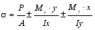1. Introduction

The foundation is the part of an engineered system that transmits to and into the underlying soil or rock the load supported by the foundation and its self-weight. The superstructure is commonly used to describe the engineered part of the system bring load to the foundations and substructures. Foundation elements must be proportioned both to interface with the soil at safe stress levels and to limit settlement to an acceptable amount

[1]

. The foundation design is assumed to be safe if the permissible stress of the soil or rock is not exceeded. The method recognizes the highly variable strength and stiffness properties of the soil or rock, as well as the important influence of such factors as the level of the groundwater and the rate of loading on strength and stiffness and possible uncertainty about the reliability of the analytical method used to calculate the failure condition of the ground

[2]

. If the foundation under consideration rests on sand or clay soil of medium compaction, an increase in the load on the foundation will also be accompanied by an increase in settlement

[3]

There are several studies that focus on optimizing the design of various footing types, including rectangular, trapezoidal, circular, and T-shaped combined footings, with an emphasis on cost efficiency, material reduction, and structural stability. Several mathematical and optimization models, including genetic algorithms, finite element methods, and boundary-type approaches, have been applied to improve load distribution, minimize contact area, and account for real soil pressure distributions. While these models enhance accuracy and reduce material use, most assume simplified soil pressure conditions, uniform load distributions, or rigid soil assumptions. Those studies are strap and combined footings, essential to support more than one column, are dealt with by

[3]

and mathematically designed by

[1]

. Practical limitations are elaborated by

[2]

, and elastic analysis is brought to light by

[4]

for optimizing the combined footing. Eccentric and boundary footings have to be redistributed carefully in pressure, and

[3]

handles axial load and moment, whereas

[1]

provides models of stability, and

[5]

handles stress and load transfer. Optimization techniques improve cost-effectiveness, as stated by

[3]

in material reduction,

[1]

in design processes, and

[6]

in computation tools.

[7]

Several models optimize footing design by incorporating real or uniform soil pressure to enhance cost efficiency and material savings. While some models improve precision by considering actual ground pressure

[8]

. others minimize contact area when pressure is uniform, limiting flexibility to complex loads and varying soil conditions

[9]

. Optimization procedures focus on rectangular, trapezoidal, and combined corner footings, reducing material but still limited to idealized soil conditions

[8]

Mathematical models optimize circular footing design through the use of real soil pressure, axial loads, and flexure, with considerable material reduction compared to traditional practice. While more efficient, the methods are applicable only to circular footings and are not as flexible to cope with intricate soil-structure interaction

[12]

. Others integrate moment and shear calculations but employ stiff soil assumptions, further restricting broader applicability.

Rectangular and trapezoidal foundation optimization designs enhance cost-effectiveness by ensuring the reduction of material usage under linear assumptions of soil pressure distribution

[14]

. They offer better solutions but are limited by idealized boundary conditions and uniform pressure assumptions, which reduce flexibility to different geometries and dynamic loads

[21]

. Nevertheless, they achieve significant reductions in material and labor costs in some foundation types.

Optimization designs of T-footings, combined footings, and rectangular pile caps enhance cost efficiency through reduced material use while maintaining structural stability

[25]

. The designs are based on actual or assumed soil pressure distribution but are restricted by assumptions of uniform loads; hence, they are not as flexible to varied soil conditions

[26]

. Despite these limitations, they still bring significant savings in material and increase load transfer efficiency in particular types of foundations.

Comparative and computational research maximizes footing design via different approaches such as trapezoidal boundary footings to reduce costs

[10]

, artificial neural networks to predict bearing capacity, and 3D FEM models to improve soil interaction precision

[27]

. Analytical and numerical methods further optimize footing dimensioning for eccentric loads, genetic algorithms minimize RCC footing costs

[11]

, and boundary-type methods enhance soil stress analysis without meshing

[29]

. Algebraic and iterative models improve precision in stress distribution but remain computationally intensive and of restricted use

[30]

Several optimization and analytical models enhance footing design efficiency. A simplified formula for sizing rectangular footings under biaxial bending accelerates design but assumes full compression. Skirted footings increase load and stability, with deeper skirts delivering better performance

[13]

. MINLP and metaheuristic algorithms optimize pad and RC footing designs to reduce cost while maximizing safety and ensuring structural integrity

[33]

. Hybrid approaches like Big Bang-Big Crunch and UPSO reduce CO₂ emissions, enhance cost savings, and improve convergence speed in optimization

[34]

. Axial load and biaxial moment interaction diagrams help estimate foundation capacity, aiding seismic design

[14]

Optimization techniques enhance reinforced concrete footing design efficiency and cost savings. Rectangular combined skirted footings reduce settlement and soil pressure and emphasize positioning skirts strategically. Genetic algorithms and metaheuristic techniques optimize spread foundation and RC footing design for maximum safety and minimum material cost

[41]

. Analytical and experimental studies confirm the soil pressure models, improving base pressure calculation accuracy and rotational spring constants for structural design

[35]

. Non-linear programming and the GRG method minimize cost-effective raft foundations and cohesive soil footings

[36]

. Shape optimization methods, including the Simplified Design Method (SDM) and Diagonal Strip Method (DSM), improve rigidity and reduce reinforcement requirements in irregular and square footings

[37]

. The Hooke & Jeeves procedure and the circular footing models enhance structure safety and material usage by means of shear force and earth pressure optimization

[38]

Experiments show that circular footings are most economical in cost owing to efficient use of contact area, whereas T-shaped footings are more material-efficient than trapezoidal footings

[39]

. Rectangular footing arrangements are improved with improved uniaxial bending models, taking into account partial soil compression, and more accurate ground pressure formulas, leading to increased material efficiency

[15]

. Square footings under general loads lead to improved material use by employing actual soil pressure instead of uniform assumptions

[16]

Strap beams reduce bending stresses and redistribute forces, improving stability, especially under seismic loads, and tie beams enhance load distribution and footing stability

[40]

. Genetic algorithm-type models reduce cost and load distribution for biaxial bending, illustrating that minimum contact area does not guarantee minimum cost. Circular foundations are even less costly than rectangular, and a novel boundary combined footing model optimizes soil pressure to achieve least material usage. Genetic algorithms also optimize eccentrically loaded footings with a focus on the impact of steel strength, concrete strength, and eccentricity in economical designs

[17]

. Comparative structural code studies of isolated footings reveal discrepancies in estimates of failure load, with a suggestion for better accuracy

[18]

Optimization methods of reinforced concrete footings include a mathematical model for corner strap combined footings under non-homogeneous ground pressure

[19]

, a spreadsheet program based on metaheuristics comprising EA and GA for isolated footings

[28]

, and a model with real soil pressure for rectangular footings

[31]

, all bringing about impressive cost savings and design enhancement. Cost reduction techniques are implemented in RC structures, shallow foundations with DE, ES, and BBO

[32]

, and high bridge piers with ant colony optimization

[20]

to achieve cost savings through optimized geometry, reinforcement, and efficiency in load distribution while maintaining safety

[21]

Metaheuristic algorithms such as HS, TLBO, and FPA continue to optimize RC footing design

[8]

, and column-reinforced foundations benefit from IAR analysis for greater bearing capacity and settlement control

[16]

. GA and UPSO-based approaches reduce costs without compromising structural safety

[22]

. A hybrid iterative method minimizes carbon footprints in RC structures by 18.3% in beams and 12% using lightweight panels

[23]

. Powell's method optimizes column footings isolated with 10%-40% cost reduction using various soil profiles

[24]

. A PSO-based method enhances the cost-effectiveness of spread footings and retaining walls

[25]

Soil pressure distribution remains a significant field of research, with

[3]

analyzing uniform, linear, and parabolic assumptions of pressure,

[1]

analyzing soil-structure interaction, and

[2]

providing empirical settlement and bearing capacity estimation procedures, all towards more accurate footing designs.

This paper introduces an innovative mathematical model for designing multigonal corner combined footings that incorporates an additional layer of flexibility: the ability for the two inner sides of the footing to be inclined linearly, allowing them to vary from 90 degrees (vertical) to 0 degrees (horizontal). This feature significantly enhances the model's adaptability to complex loading conditions and site constraints, while optimizing the footing's geometry and load distribution.

The model emphasizes the optimization of footing sizes to reduce construction costs while ensuring structural stability. The critical parameters to be taken into account are the load-carrying capacity of the soil (σall), the impact of axial loads and biaxial bending moments, and the location of the load center relative to the geometric center of the footing. By considering these parameters, the model attempts to create cost-effective and efficient foundation designs that are safe and perform well.

2. Materials and Methods

The method used for this study is to define the geometry of multigonal corner combined footings and establish key parameters such as structural loads and soil bearing capacities. Mathematical models are developed to demonstrate the design constraints, including bearing capacity and stress distribution. Mathematical explanations are done using Maple, and Python is used to create a numerical optimization model. Verification is done using Python to verify the accuracy of the developed model. In addition, a parametric analysis is performed to determine how the design variables respond to variations in the input parameters.

The universal formula for footings of any kind that are bent in both directions.

(1)

Where: σ is the soil pressure stress exerted on the footing; A is the footing's contact area; P is the axial load applied at the footing's center of gravity; Mx and My are the moments around the axes “X and Y”, respectively; x and y are the distances in the direction of “X” measured from the axis “Y” to the fiber under study and the farthest under study, respectively; Iy and Ix are the moments of inertia around the axis “Y” and the moment of inertia around the axis “X”.

The pressure below the combined footing in each column of Figure 1 is subject to a linear variation under axial load and moment in two directions (biaxial bending).

Download: Download full-size image

Figure 1. Corner multi-gonal footing.

The pressure diagram beneath the corner combined footing and the stresses in each vertex are displayed in Figure 2.

Download: Download full-size image

Figure 2. Pressure diagram below the footing.

From the eq. (1), the stresses in each vertex of the footing are obtained

σ_{1} = \frac{R}{A} + \frac{M_{xt} \cdot y_{b}}{I_{x}} + \frac{M_{yt} \cdot x_{b}}{I_{y}}

(2)

σ_{2} = \frac{R}{A} + \frac{M_{xt} \cdot y_{b}}{I_{x}} - \frac{M_{yt} \cdot (a - x_{b})}{I_{y}}

(3)

σ_{3} = \frac{R}{A} + \frac{M_{xt} \cdot (y_{b} - b_{1} - m)}{I_{x}} + \frac{M_{yt} \cdot (x_{b} - b_{2} - n)}{I_{y}}

(4)

σ_{4} = \frac{R}{A} + \frac{M_{xt} \cdot (y_{b} - b_{1})}{I_{x}} - \frac{M_{yt} \cdot (a - x_{b})}{I_{y}}

(5)

σ_{5} = \frac{R}{A} - \frac{M_{xt} \cdot (b - y_{b})}{I_{x}} + \frac{M_{yt} \cdot x_{b}}{I_{y}}

(6)

σ_{6} = \frac{R}{A} - \frac{M_{xt} \cdot (b - y_{b})}{I_{x}} + \frac{M_{yt} \cdot (x_{b} - b_{2})}{I_{y}}

(7)

R = P_{1} + P_{2} + P_{3}

(8)

M_{xt} = M_{x 1} + M_{x 2} + M_{x 3} + P_{1} (y_{b} - \frac{c_{3}}{2}) + P_{2} (y_{b} - \frac{c_{3}}{2}) - P_{3} (L_{2} + \frac{c_{3}}{2} - y_{b})

(9)

M_{yt} = M_{y 1} + M_{y 2} + M_{y 3} + P_{1} (x_{b} - \frac{c_{1}}{2}) - P_{2} (L_{1} + \frac{c_{1}}{2} - x_{b}) + P_{3} (x_{b} - \frac{c_{1}}{2})

(10)

A = \frac{(2 a - n - 2 b_{2}) b_{1}}{2} + \frac{(2 b - m) b_{2}}{2} + \frac{ma}{2} + \frac{nb}{2}

(11)

x_{b} = \frac{(3 b - 2 m - 3 b_{1}) {b_{2}}^{2} + ((3 b - m - 3 b_{1}) n + ma) b_{2} + (b - b_{1}) n^{2} + man + a^{2} (m + 3 b_{1})}{(6 b - 3 m - 6 b_{1}) b_{2} + (3 b - 3 b_{1}) n + 3 a (m + 2 b_{1})}

(12)

y_{b} = \frac{(3 a - 2 n - 3 b_{2}) {b_{1}}^{2} + ((3 a - n - 3 b_{2}) m + nb) b_{1} + (a - b_{2}) m^{2} + nbm + b^{2} (3 b_{2} + n)}{(6 a - 3 n - 6 b_{2}) b_{1} + (3 a - 3 b_{2}) m + 3 b (2 b_{2} + n)}

(13)

I_{x} = \begin{matrix} [\frac{b_{2} b^{3}}{12} + b b_{2} {(y_{b} - \frac{b}{2})}^{2}] + [\frac{(a - b_{2}) b_{1}^{3}}{12} + (a - b_{2}) b_{1} {(y_{b} - \frac{b_{1}}{2})}^{2}] \\ + [\frac{n m^{3}}{12} + nm {(y_{b} - b_{1} - \frac{m}{2})}^{2}] + [\frac{(a - b_{2} - n) m^{3}}{36} + \frac{(a - b_{2} - n) m}{2} {(y_{b} - b_{1} - \frac{m}{3})}^{2}] \\ + [\frac{n (b - b_{1} - m)^{3}}{36} + \frac{(b - b_{1} - m) n}{2} {(y_{b} - \frac{2 b_{1} + 2 m + b}{3})}^{2}] \end{matrix}

(14)

I_{y} = \begin{matrix} [\frac{b b_{2}^{3}}{12} + b b_{2} {(x_{b} - \frac{b_{2}}{2})}^{2}] + [\frac{(a - b_{2})^{3} b_{1}}{12} + (a - b_{2}) b_{1} {(x_{b} - \frac{b_{2} + a}{2})}^{2}] \\ + [\frac{n^{3} m}{12} + nm {(x_{b} - b_{2} - \frac{n}{2})}^{2}] + [\frac{(a - b_{2} - n)^{3} m}{36} + \frac{(a - b_{2} - n) m}{2} {(x_{b} - b_{2} - n - \frac{a - b_{2} - n}{3})}^{2}] \\ + [\frac{n^{3} (b - b_{1} - m)}{36} + \frac{(b - b_{1} - m) n}{2} {(x_{b} - b_{2} - \frac{n}{3})}^{2}] \end{matrix}

(15)

σ_{1} = \begin{matrix} \frac{P_{1} + P_{2} + P_{3}}{b b_{2} + (a - b_{2}) b_{1} + nm + \frac{(a - b_{2} - n) m}{2} + \frac{(b - b_{1} - m) n}{2}} \\ + \frac{1}{I_{x}} [M_{x 1} + M_{x 2} + M_{x 3} - \frac{(P_{1} + P_{2} + P_{3}) c_{3}}{2} - P_{3} L_{2} \\ + \frac{P_{1} + P_{2} + P_{3}}{b b_{2} + (a - b_{2}) b_{1} + nm + \frac{(a - b_{2} - n) m}{2} + \frac{(b - b_{1} - m) n}{2}} \cdot (\frac{b^{2} b_{2}}{2} + \frac{(a - b_{2}) b_{1}^{2}}{2} + nm (b_{1} + \frac{m}{2}) + \frac{(a - b_{2} - n) m (b_{1} + \frac{m}{3})}{2} + \frac{(b - b_{1} - m) n (\frac{2 b_{1} + 2 m + b}{3})}{2})] \\ \cdot \frac{\frac{b^{2} b_{2}}{2} + \frac{(a - b_{2}) b_{1}^{2}}{2} + nm (b_{1} + \frac{m}{2}) + \frac{(a - b_{2} - n) m (b_{1} + \frac{m}{3})}{2} + \frac{(b - b_{1} - m) n (\frac{2 b_{1} + 2 m + b}{3})}{2}}{b b_{2} + (a - b_{2}) b_{1} + nm + \frac{(a - b_{2} - n) m}{2} + \frac{(b - b_{1} - m) n}{2}} \\ + \frac{1}{I_{y}} [M_{y 1} + M_{y 2} + M_{y 3} - \frac{(P_{1} + P_{2} + P_{3}) c_{1}}{2} - P_{2} L_{1} \\ + \frac{P_{1} + P_{2} + P_{3}}{b b_{2} + (a - b_{2}) b_{1} + nm + \frac{(a - b_{2} - n) m}{2} + \frac{(b - b_{1} - m) n}{2}} \cdot (\frac{b b_{2}^{2}}{2} + (a - b_{2}) b_{1} (\frac{b_{2} + a}{2}) + nm (b_{2} + \frac{n}{2}) + \frac{(a - b_{2} - n) m (\frac{2 b_{2} + 2 n + a}{3})}{2} + \frac{(b - b_{1} - m) n (b_{2} + \frac{n}{3})}{2})] \\ \cdot \frac{\frac{b b_{2}^{2}}{2} + (a - b_{2}) b_{1} (\frac{b_{2} + a}{2}) + nm (b_{2} + \frac{n}{2}) + \frac{(a - b_{2} - n) m (\frac{2 b_{2} + 2 n + a}{3})}{2} + \frac{(b - b_{1} - m) n (b_{2} + \frac{n}{3})}{2}}{b b_{2} + (a - b_{2}) b_{1} + nm + \frac{(a - b_{2} - n) m}{2} + \frac{(b - b_{1} - m) n}{2}} \end{matrix}

(16)

σ_{2} = \begin{matrix} \frac{P_{1} + P_{2} + P_{3}}{b b_{2} + (a - b_{2}) b_{1} + nm + \frac{(a - b_{2} - n) m}{2} + \frac{(b - b_{1} - m) n}{2}} \\ + \frac{1}{I_{x}} [M_{x 1} + M_{x 2} + M_{x 3} - \frac{(P_{1} + P_{2} + P_{3}) c_{3}}{2} - P_{3} L_{2} \\ + \frac{P_{1} + P_{2} + P_{3}}{b b_{2} + (a - b_{2}) b_{1} + nm + \frac{(a - b_{2} - n) m}{2} + \frac{(b - b_{1} - m) n}{2}} \cdot (\frac{b^{2} b_{2}}{2} + \frac{(a - b_{2}) b_{1}^{2}}{2} + nm (b_{1} + \frac{m}{2}) + \frac{(a - b_{2} - n) m (b_{1} + \frac{m}{3})}{2} + \frac{(b - b_{1} - m) n (\frac{2 b_{1} + 2 m + b}{3})}{2})] \\ \cdot \frac{\frac{b^{2} b_{2}}{2} + \frac{(a - b_{2}) b_{1}^{2}}{2} + nm (b_{1} + \frac{m}{2}) + \frac{(a - b_{2} - n) m (b_{1} + \frac{m}{3})}{2} + \frac{(b - b_{1} - m) n (\frac{2 b_{1} + 2 m + b}{3})}{2}}{b b_{2} + (a - b_{2}) b_{1} + nm + \frac{(a - b_{2} - n) m}{2} + \frac{(b - b_{1} - m) n}{2}} \\ - \frac{1}{I_{y}} [M_{y 1} + M_{y 2} + M_{y 3} - \frac{(P_{1} + P_{2} + P_{3}) c_{1}}{2} - P_{2} L_{1} \\ + \frac{P_{1} + P_{2} + P_{3}}{b b_{2} + (a - b_{2}) b_{1} + nm + \frac{(a - b_{2} - n) m}{2} + \frac{(b - b_{1} - m) n}{2}} \cdot (\frac{b b_{2}^{2}}{2} + (a - b_{2}) b_{1} (\frac{b_{2} + a}{2}) + nm (b_{2} + \frac{n}{2}) + \frac{(a - b_{2} - n) m (\frac{2 b_{2} + 2 n + a}{3})}{2} + \frac{(b - b_{1} - m) n (b_{2} + \frac{n}{3})}{2})] \\ \cdot (a - \frac{\frac{b b_{2}^{2}}{2} + (a - b_{2}) b_{1} (\frac{b_{2} + a}{2}) + nm (b_{2} + \frac{n}{2}) + \frac{(a - b_{2} - n) m (\frac{2 b_{2} + 2 n + a}{3})}{2} + \frac{(b - b_{1} - m) n (b_{2} + \frac{n}{3})}{2}}{b b_{2} + (a - b_{2}) b_{1} + nm + \frac{(a - b_{2} - n) m}{2} + \frac{(b - b_{1} - m) n}{2}}) \end{matrix}

(17)

σ_{3} = \begin{matrix} \frac{P_{1} + P_{2} + P_{3}}{b b_{2} + (a - b_{2}) b_{1} + nm + \frac{(a - b_{2} - n) m}{2} + \frac{(b - b_{1} - m) n}{2}} \\ + \frac{1}{I_{x}} [M_{x 1} + M_{x 2} + M_{x 3} - \frac{(P_{1} + P_{2} + P_{3}) c_{3}}{2} - P_{3} L_{2} \\ + \frac{P_{1} + P_{2} + P_{3}}{b b_{2} + (a - b_{2}) b_{1} + nm + \frac{(a - b_{2} - n) m}{2} + \frac{(b - b_{1} - m) n}{2}} \cdot (\frac{b^{2} b_{2}}{2} + \frac{(a - b_{2}) b_{1}^{2}}{2} + nm (b_{1} + \frac{m}{2}) + \frac{(a - b_{2} - n) m (b_{1} + \frac{m}{3})}{2} + \frac{(b - b_{1} - m) n (\frac{2 b_{1} + 2 m + b}{3})}{2})] \\ \cdot (\frac{\frac{b^{2} b_{2}}{2} + \frac{(a - b_{2}) b_{1}^{2}}{2} + nm (b_{1} + \frac{m}{2}) + \frac{(a - b_{2} - n) m (b_{1} + \frac{m}{3})}{2} + \frac{(b - b_{1} - m) n (\frac{2 b_{1} + 2 m + b}{3})}{2}}{b b_{2} + (a - b_{2}) b_{1} + nm + \frac{(a - b_{2} - n) m}{2} + \frac{(b - b_{1} - m) n}{2}} - b_{1} - m) \\ + \frac{1}{I_{y}} [M_{y 1} + M_{y 2} + M_{y 3} - \frac{(P_{1} + P_{2} + P_{3}) c_{1}}{2} - P_{2} L_{1} \\ + \frac{P_{1} + P_{2} + P_{3}}{b b_{2} + (a - b_{2}) b_{1} + nm + \frac{(a - b_{2} - n) m}{2} + \frac{(b - b_{1} - m) n}{2}} \cdot (\frac{b b_{2}^{2}}{2} + (a - b_{2}) b_{1} (\frac{b_{2} + a}{2}) + nm (b_{2} + \frac{n}{2}) + \frac{(a - b_{2} - n) m (\frac{2 b_{2} + 2 n + a}{3})}{2} + \frac{(b - b_{1} - m) n (b_{2} + \frac{n}{3})}{2})] \\ \cdot (\frac{\frac{b b_{2}^{2}}{2} + (a - b_{2}) b_{1} (\frac{b_{2} + a}{2}) + nm (b_{2} + \frac{n}{2}) + \frac{(a - b_{2} - n) m (\frac{2 b_{2} + 2 n + a}{3})}{2} + \frac{(b - b_{1} - m) n (b_{2} + \frac{n}{3})}{2}}{b b_{2} + (a - b_{2}) b_{1} + nm + \frac{(a - b_{2} - n) m}{2} + \frac{(b - b_{1} - m) n}{2}} - b_{2} - n) \end{matrix}

(18)

σ_{4} = \begin{matrix} \frac{P_{1} + P_{2} + P_{3}}{b b_{2} + (a - b_{2}) b_{1} + nm + \frac{(a - b_{2} - n) m}{2} + \frac{(b - b_{1} - m) n}{2}} \\ + \frac{1}{I_{x}} [M_{x 1} + M_{x 2} + M_{x 3} - \frac{(P_{1} + P_{2} + P_{3}) c_{3}}{2} - P_{3} L_{2} \\ + \frac{P_{1} + P_{2} + P_{3}}{b b_{2} + (a - b_{2}) b_{1} + nm + \frac{(a - b_{2} - n) m}{2} + \frac{(b - b_{1} - m) n}{2}} \cdot (\frac{b^{2} b_{2}}{2} + \frac{(a - b_{2}) b_{1}^{2}}{2} + nm (b_{1} + \frac{m}{2}) + \frac{(a - b_{2} - n) m (b_{1} + \frac{m}{3})}{2} + \frac{(b - b_{1} - m) n (\frac{2 b_{1} + 2 m + b}{3})}{2})] \\ \cdot (\frac{\frac{b^{2} b_{2}}{2} + \frac{(a - b_{2}) b_{1}^{2}}{2} + nm (b_{1} + \frac{m}{2}) + \frac{(a - b_{2} - n) m (b_{1} + \frac{m}{3})}{2} + \frac{(b - b_{1} - m) n (\frac{2 b_{1} + 2 m + b}{3})}{2}}{b b_{2} + (a - b_{2}) b_{1} + nm + \frac{(a - b_{2} - n) m}{2} + \frac{(b - b_{1} - m) n}{2}} - b_{1}) \\ - \frac{1}{I_{y}} [M_{y 1} + M_{y 2} + M_{y 3} - \frac{(P_{1} + P_{2} + P_{3}) c_{1}}{2} - P_{2} L_{1} \\ + \frac{P_{1} + P_{2} + P_{3}}{b b_{2} + (a - b_{2}) b_{1} + nm + \frac{(a - b_{2} - n) m}{2} + \frac{(b - b_{1} - m) n}{2}} \cdot (\frac{b b_{2}^{2}}{2} + (a - b_{2}) b_{1} (\frac{b_{2} + a}{2}) + nm (b_{2} + \frac{n}{2}) + \frac{(a - b_{2} - n) m (\frac{2 b_{2} + 2 n + a}{3})}{2} + \frac{(b - b_{1} - m) n (b_{2} + \frac{n}{3})}{2})] \\ \cdot (a - \frac{\frac{b b_{2}^{2}}{2} + (a - b_{2}) b_{1} (\frac{b_{2} + a}{2}) + n m (b_{2} + \frac{n}{2}) + \frac{(a - b_{2} - n) m (\frac{2 b_{2} + 2 n + a}{3})}{2} + \frac{(b - b_{1} - m) n (b_{2} + \frac{n}{3})}{2}}{b b_{2} + (a - b_{2}) b_{1} + nm + \frac{(a - b_{2} - n) m}{2} + \frac{(b - b_{1} - m) n}{2}}) \end{matrix}

(19)

σ_{5} = \begin{matrix} \frac{P_{1} + P_{2} + P_{3}}{b b_{2} + (a - b_{2}) b_{1} + nm + \frac{(a - b_{2} - n) m}{2} + \frac{(b - b_{1} - m) n}{2}} \\ - \frac{1}{I_{x}} [M_{x 1} + M_{x 2} + M_{x 3} - \frac{(P_{1} + P_{2} + P_{3}) c_{3}}{2} - P_{3} L_{2} \\ + \frac{P_{1} + P_{2} + P_{3}}{b b_{2} + (a - b_{2}) b_{1} + nm + \frac{(a - b_{2} - n) m}{2} + \frac{(b - b_{1} - m) n}{2}} \cdot (\frac{b^{2} b_{2}}{2} + \frac{(a - b_{2}) b_{1}^{2}}{2} + nm (b_{1} + \frac{m}{2}) + \frac{(a - b_{2} - n) m (b_{1} + \frac{m}{3})}{2} + \frac{(b - b_{1} - m) n (\frac{2 b_{1} + 2 m + b}{3})}{2})] \\ \cdot (b - \frac{\frac{b^{2} b_{2}}{2} + \frac{(a - b_{2}) b_{1}^{2}}{2} + nm (b_{1} + \frac{m}{2}) + \frac{(a - b_{2} - n) m (b_{1} + \frac{m}{3})}{2} + \frac{(b - b_{1} - m) n (\frac{2 b_{1} + 2 m + b}{3})}{2}}{b b_{2} + (a - b_{2}) b_{1} + nm + \frac{(a - b_{2} - n) m}{2} + \frac{(b - b_{1} - m) n}{2}}) \\ + \frac{1}{I_{y}} [M_{y 1} + M_{y 2} + M_{y 3} - \frac{(P_{1} + P_{2} + P_{3}) c_{1}}{2} - P_{2} L_{1} \\ + \frac{P_{1} + P_{2} + P_{3}}{b b_{2} + (a - b_{2}) b_{1} + nm + \frac{(a - b_{2} - n) m}{2} + \frac{(b - b_{1} - m) n}{2}} \cdot (\frac{b b_{2}^{2}}{2} + (a - b_{2}) b_{1} (\frac{b_{2} + a}{2}) + nm (b_{2} + \frac{n}{2}) + \frac{(a - b_{2} - n) m (\frac{2 b_{2} + 2 n + a}{3})}{2} + \frac{(b - b_{1} - m) n (b_{2} + \frac{n}{3})}{2})] \\ \cdot \frac{\frac{b b_{2}^{2}}{2} + (a - b_{2}) b_{1} (\frac{b_{2} + a}{2}) + nm (b_{2} + \frac{n}{2}) + \frac{(a - b_{2} - n) m (\frac{2 b_{2} + 2 n + a}{3})}{2} + \frac{(b - b_{1} - m) n (b_{2} + \frac{n}{3})}{2}}{b b_{2} + (a - b_{2}) b_{1} + nm + \frac{(a - b_{2} - n) m}{2} + \frac{(b - b_{1} - m) n}{2}} \end{matrix}

(20)

σ_{6} = \begin{matrix} \frac{P_{1} + P_{2} + P_{3}}{b b_{2} + (a - b_{2}) b_{1} + nm + \frac{(a - b_{2} - n) m}{2} + \frac{(b - b_{1} - m) n}{2}} \\ - \frac{1}{I_{x}} [M_{x 1} + M_{x 2} + M_{x 3} - \frac{(P_{1} + P_{2} + P_{3}) c_{3}}{2} - P_{3} L_{2} \\ + \frac{P_{1} + P_{2} + P_{3}}{b b_{2} + (a - b_{2}) b_{1} + nm + \frac{(a - b_{2} - n) m}{2} + \frac{(b - b_{1} - m) n}{2}} \cdot (\frac{b^{2} b_{2}}{2} + \frac{(a - b_{2}) b_{1}^{2}}{2} + nm (b_{1} + \frac{m}{2}) + \frac{(a - b_{2} - n) m (b_{1} + \frac{m}{3})}{2} + \frac{(b - b_{1} - m) n (\frac{2 b_{1} + 2 m + b}{3})}{2})] \\ \cdot (b - \frac{\frac{b^{2} b_{2}}{2} + \frac{(a - b_{2}) b_{1}^{2}}{2} + nm (b_{1} + \frac{m}{2}) + \frac{(a - b_{2} - n) m (b_{1} + \frac{m}{3})}{2} + \frac{(b - b_{1} - m) n (\frac{2 b_{1} + 2 m + b}{3})}{2}}{b b_{2} + (a - b_{2}) b_{1} + nm + \frac{(a - b_{2} - n) m}{2} + \frac{(b - b_{1} - m) n}{2}}) \\ + \frac{1}{I_{y}} [M_{y 1} + M_{y 2} + M_{y 3} - \frac{(P_{1} + P_{2} + P_{3}) c_{1}}{2} - P_{2} L_{1} \\ + \frac{P_{1} + P_{2} + P_{3}}{b b_{2} + (a - b_{2}) b_{1} + nm + \frac{(a - b_{2} - n) m}{2} + \frac{(b - b_{1} - m) n}{2}} \cdot (\frac{b b_{2}^{2}}{2} + (a - b_{2}) b_{1} (\frac{b_{2} + a}{2}) + nm (b_{2} + \frac{n}{2}) + \frac{(a - b_{2} - n) m (\frac{2 b_{2} + 2 n + a}{3})}{2} + \frac{(b - b_{1} - m) n (b_{2} + \frac{n}{3})}{2})] \\ \cdot (\frac{\frac{b b_{2}^{2}}{2} + (a - b_{2}) b_{1} (\frac{b_{2} + a}{2}) + nm (b_{2} + \frac{n}{2}) + \frac{(a - b_{2} - n) m (\frac{2 b_{2} + 2 n + a}{3})}{2} + \frac{(b - b_{1} - m) n (b_{2} + \frac{n}{3})}{2}}{b b_{2} + (a - b_{2}) b_{1} + nm + \frac{(a - b_{2} - n) m}{2} + \frac{(b - b_{1} - m) n}{2}} - b_{2}) \end{matrix}

(21)

Numerical Problems

The tables show five scenarios for dimensioning corner combined footings with two adjacent boundaries. Each scenario varies the soil's allowable load capacity, with values of "σall = 200, 250, 300, 350, 400 kN/m²". Within each scenario, there are four types of multigonal corner combined footings presented, each type differing in the mechanical elements acting on the footing. These four types, detailed in Table 1, remain consistent across all scenarios.

Table 1. Mechanical elements acting on the footing.

Type	Loads of column 1			Loads of column 2			Loads of column 3			Load center
Type	P1 kN	Mx1 kN-m	_My1 kN-m	P2 kN	Mx2 kN-m	My2 kN-m	P3 kN	Mx3 kN-m	My3 kN-m	X(m)	Y(m)
1	700	200	150	1200	250	350	1000	300	300	2.20	1.67
2	700	-200	150	1200	-250	350	1000	-300	300	2.20	2.18
3	700	200	-150	1200	250	-350	1000	300	-300	2.75	1.67
4	700	-200	-150	1200	-250	-350	1000	-300	-300	2.75	2.18

Additionally, Table 2 investigates how the dimensions of the footing are impacted by increasing the load at the corner. It provides insights into the required footing dimensions under two conditions: when the parameters “n” and “m” are both set to 0, and when “n” and “m” are greater than 0. This additional analysis helps to understand how variations in corner load influence dimensioning of multigonal corner combined footings across different soil load-bearing capacities and mechanical configurations. For the dimensions b1<0.4 and b2<0.4 in this condition, the results are favorable to "n" and "m" having greater than zero; nevertheless, these dimensions are not helpful in real-world applications. Consequently, b1 and b2 are restricted to a minimum of 0.4 meters in order to ensure design feasibility.

Table 2. Mechanical elements acting on the footing with increasing load at the corner column.

Type	Loads of column 1			Loads of column 2			Loads of column 3			Load center
Type	P1 kN	Mx1 kN-m	My1 kN-m	P2 kN	Mx2 kN-m	My2 kN-m	P3 kN	Mx3 kN-m	My3 kN-m	X(m)	Y(m)
1	1200	200	150	800	250	350	900	300	300	1.44	1.53
2	1200	-200	150	800	-250	350	900	-300	300	1.44	1.98
3	1200	200	-150	800	250	-350	900	300	-300	1.99	1.53
4	1200	-200	-150	800	-250	-350	900	-300	-300	1.99	1.98

The results were displayed in Tables 3, 4, 5, 6, 7 and 8, the result of tables 3, 4, 5, and 6 corresponds to the loading condition of table 1 and the result of table 7 and 8 corresponds to the loading condition of table 2 which also included the following considerations: 1) The three columns' dimensions are 40 by 40 cm in every scenario; 2) Each situation has a different soil allowed load bearing capacity; The separation of columns is L1 = 5.50 m and L2 = 5.00 m.

The results of the optimization techniques are displayed in Tables 3, 4, 5, 6, 7 and 8. The Python software is used to determine the minimum areas and dimensions for multigonal corner combined footings, and it is assumed that the dimensions are non-negative. The objective function (minimum contact surface) is obtained by Eq. (11), and constraint functions by Eqs. (16) to (21) are found.

P1, Mx1, My1, P2, Mx2, My2, P3, Mx3, My3, n, m, c1, c2, c3, c4, L1, L2, σall, R are the constant parameters assumed in this issue, and the decision variables are MxT, MyT, a, b, b1, b2, σ1, σ2, σ3, σ4, σ5, σ6.

Table 3 takes into account the following factors: MxT and MyT are unconstrained, R=2900 kN There are 5.90 m≤a, 5.40 m≤b, 0≤b1, 0≤b2, 0≤n, 0≤m, when it comes to its goal function, 0≤σ1≤σall, 0≤σ2≤σall, 0≤σ3≤σall, 0≤σ4≤σall, 0≤σ5≤σall, 0≤σ6≤σall. Table 4 takes into account the following factors: MxT and MyT are unconstrained, R=2900 kN There are 5.90 m≤a, 5.40 m≤b, 0.5≤b1, 0.5≤b2, 0≤n, 0≤m, when it comes to its goal function, 0≤σ1≤σall, 0≤σ2≤σall, 0≤σ3≤σall, 0≤σ4≤σall, 0≤σ5≤σall, 0≤σ6≤σall. Table 5 takes into account the following factors: MxT and MyT are unconstrained, R=2900 kN There are 5.90 m≤a, 5.40 m≤b, 1≤b1, 1≤b2, 0≤n, 0≤m, when it comes to its goal function, 0≤σ1≤σall, 0≤σ2≤σall, 0≤σ3≤σall, 0≤σ4≤σall, 0≤σ5≤σall, 0≤σ6≤σall. Table 6 takes into account the following factors: MxT and MyT are unconstrained, R=2900 kN There are 5.90 m=a, 5.40 m=b, 0≤b1, 0≤b2, 0≤n, 0≤m, when it comes to its goal function, 0≤σ1≤σall, 0≤σ2≤σall, 0≤σ3≤σall, 0≤σ4≤σall, 0≤σ5≤σall, 0≤σ6≤σall. Table 7 takes into account the following factors: MxT and MyT are unconstrained, R=2900 kN There are 5.90 m≤a, 5.40 m≤b, 0.5≤b1, 0.5≤b2, 0=n, 0=m, when it comes to its goal function, 0≤σ1≤σall, 0≤σ2≤σall, 0≤σ3≤σall, 0≤σ4≤σall, 0≤σ5≤σall, 0≤σ6≤σall. Table 8 takes into account the following factors: MxT and MyT are unconstrained, R=2900 kN There are 5.90 m≤a, 5.40 m≤b, 0.4≤b1, 0.4≤b2, 0≤n, 0≤m, when it comes to its goal function, 0≤σ1≤σall, 0≤σ2≤σall, 0≤σ3≤σall, 0≤σ4≤σall, 0≤σ5≤σall, 0≤σ6≤σall.

Table 3. Results obtained by software for a≥5.9, b≥5.4, b1≥0, b2≥0, n≥0 and m≥0.

Type	Sum of loads and moments			Optimal area (m²)	Dimension of the footing(m)						Struss generated by loads in each corned(kN/m²)						Geometric center
Type	F_R kN	MxT kN-m	MyT kN-m	A_t	a	b	b₁	b₂	n	m	σ₁	σ₂	σ₃	σ₄	σ₅	σ₆	X(m)	Y(m)
σ_all=200.00 kN/m²
1	2900	0.00	0.00	14.50	7.17	6.65	0.26	0.61	0.11	2.55	200.00	200.00	200.00	200.00	200.00	200.00	2.20	1.67
2	2900	0.00	0.00	14.50	7.17	10.27	0.57	0.43	0.05	1.80	200.00	200.00	200.00	200.00	200.00	200.00	2.20	2.18
3	2900	0.00	0.00	14.50	9.82	6.81	0.28	0.77	0.134	1.39	200.00	200.00	200.00	200.00	200.00	200.00	2.75	1.67
4	2900	0.00	0.00	14.50	10.13	10.24	0.26	0.49	0.05	1.40	200.00	200.00	200.00	200.00	200.00	200.00	2.75	2.18
σ_all=250.00 kN/m²
1	2900	0.00	0.00	11.60	7.75	7.68	0.32	0.43	0.12	1.56	250.00	250.00	250.00	250.00	250.00	250.00	2.20	1.67
2	2900	0.00	0.00	11.60	7.92	9.57	0.41	0.44	0.09	1.04	250.00	250.00	250.00	250.00	250.00	250.00	2.20	2.18
3	2900	0.00	0.00	11.60	8.78	8.87	0.45	0.35	0.09	1.02	250.00	250.00	250.00	250.00	250.00	250.00	2.75	1.67
4	2900	0.00	0.00	11.60	10.20	10.83	0.27	0.33	0.14	0.94	250.00	250.00	250.00	250.00	250.00	250.00	2.75	2.18
σ_all=300.00 kN/m²
1	2900	0.00	0.00	9.66	7.95	7.12	0.31	0.49	0.11	0.93	300.00	300.00	300.00	300.00	300.00	300.00	2.20	1.67
2	2900	0.00	0.00	9.66	8.11	9.40	0.37	0.41	0.03	0.73	300.00	300.00	300.00	300.00	300.00	300.00	2.20	2.18
3	2900	0.00	0.00	9.66	9.09	8.20	0.44	0.35	0.17	0.52	300.00	300.00	300.00	300.00	300.00	300.00	2.75	1.67
4	2900	0.00	0.00	9.66	9.59	11.39	0.37	0.24	0.15	0.57	300.00	300.00	300.00	300.00	300.00	300.00	2.75	2.18
σ_all=350.00 kN/m²
1	2900	0.00	0.00	8.29	7.86	8.07	0.27	0.32	0.11	0.86	350.00	350.00	350.00	350.00	350.00	350.00	2.20	1.67
2	2900	0.00	0.00	8.29	8.41	9.58	0.30	0.33	0.10	0.56	350.00	350.00	350.00	350.00	350.00	350.00	2.20	2.18
3	2900	0.00	0.00	8.29	9.38	9.36	0.28	0.23	0.11	0.67	350.00	350.00	350.00	350.00	350.00	350.00	2.75	1.67
4	2900	0.00	0.00	8.29	9.79	10.88	0.29	0.28	0.01	0.53	350.00	350.00	350.00	350.00	350.00	350.00	2.75	2.18
σ_all=400.00 kN/m²
1	2900	0.00	0.00	7.25	7.20	7.85	0.50	0.29	0.17	0.28	400.00	400.00	400.00	400.00	400.00	400.00	2.20	1.67
2	2900	0.00	0.00	7.25	8.05	9.79	0.36	0.26	0.12	0.32	400.00	400.00	400.00	400.00	400.00	400.00	2.20	2.18
3	2900	0.00	0.00	7.25	9.21	8.94	0.33	0.22	0.13	0.39	400.00	400.00	400.00	400.00	400.00	400.00	2.75	1.67
4	2900	0.00	0.00	7.25	10.21	10.39	0.26	0.25	0.08	0.35	400.00	400.00	400.00	400.00	400.00	400.00	2.75	2.18

Table 4. Results obtained by software for a≥5.9, b≥5.4, b1≥0.5, b2≥0.5, n≥0 and m≥0.

Type	Sum of loads and moments			Optimal area (m²)	Dimension of the footing(m)						Struss generated by loads in each corned(kN/m²)						Geometric center
Type	F_R kN	MxT kN-m	MyT kN-m	A_t	a	b	b₁	b₂	n	m	σ₁	σ₂	σ₃	σ₄	σ₅	σ₆	X(m)	Y(m)
σ_all=200.00 kN/m²
1	2900	0.00	0.00	14.50	5.91	5.43	1.56	1.09	0.18	0.29	200.00	200.00	200.00	200.00	200.00	200.00	2.20	1.67
2	2900	0.00	0.00	14.50	7.73	8.88	0.52	0.64	0.15	1.32	200.00	200.00	200.00	200.00	200.00	200.00	2.20	2.18
3	2900	0.00	0.00	14.50	7.37	6.82	1.41	0.75	0.00	0.01	200.00	200.00	200.00	200.00	200.00	200.00	2.75	1.67
4	2900	0.00	0.00	14.50	9.40	7.81	0.79	0.94	0.00	0.10	200.00	200.00	200.00	200.00	200.00	200.00	2.75	2.18
σ_all=250.00 kN/m²
1	2900	0.00	0.00	11.60	7.21	5.57	0.81	1.03	0.16	0.15	250.00	250.00	250.00	250.00	250.00	250.00	2.20	1.67
2	2900	0.00	0.00	11.60	8.76	7.13	0.51	0.90	0.11	0.22	250.00	250.00	250.00	250.00	250.00	250.00	2.20	2.18
3	2900	0.00	0.00	11.60	8.41	6.68	0.82	0.73	0.01	0.09	250.00	250.00	250.00	250.00	250.00	250.00	2.75	1.67
4	2900	0.00	0.00	11.60	10.11	8.72	0.50	0.53	0.25	0.24	250.00	250.00	250.00	250.00	250.00	250.00	2.75	2.18
σ_all=300.00 kN/m²
1	2900	0.00	0.00	9.66	7.04	6.46	0.73	0.64	0.08	0.20	300.00	300.00	300.00	300.00	300.00	300.00	2.20	1.67
2	2900	0.00	0.00	9.66	8.10	8.23	0.53	0.54	0.11	0.21	300.00	300.00	300.00	300.00	300.00	300.00	2.20	2.18
3	2900	0.00	0.00	9.66	8.87	6.76	0.61	0.63	0.00	0.09	300.00	300.00	300.00	300.00	300.00	300.00	2.75	1.67
4	2900	0.00	0.00	9.66	10.03	8.04	0.50	0.62	0.00	0.00	300.00	300.00	300.00	300.00	300.00	300.00	2.75	2.18
σ_all=350.00 kN/m²
1	2900	0.00	0.00	8.29	7.43	6.70	0.53	0.52	0.07	0.26	350.00	350.00	350.00	350.00	350.00	350.00	2.20	1.67
2	2900	0.00	0.00	8.29	8.12	8.05	0.51	0.50	0.07	0.02	350.00	350.00	350.00	350.00	350.00	350.00	2.20	2.18
3	2900	0.00	0.00	8.29	8.85	6.93	0.56	0.52	0.01	0.00	350.00	350.00	350.00	350.00	350.00	350.00	2.75	1.67
4	2900	-165.19	-197.26	8.59	9.40	8.28	0.50	0.50	0.00	0.00	324.40	348.53	327.15	350.00	348.72	350.00	2.68	2.13
σ_all=400.00 kN/m²
1	2900	0.00	0.00	7.25	7.53	6.28	0.53	0.55	0.03	0.00	400.00	400.00	400.00	400.00	400.00	400.00	2.20	1.67
2	2900	-172.05	-173.19	7.54	7.81	7.77	0.50	0.50	0.00	0.00	368.04	398.01	371.90	400.00	398.08	400.00	2.14	2.12
3	2900	-117.56	-173.34	7.50	8.81	6.67	0.50	0.50	0.00	0.00	372.57	398.01	375.97	400.00	398.56	400.00	2.69	1.62
4	2900	-490.65	-587.71	8.10	8.88	7.81	0.50	0.50	0.00	0.00	313.86	394.78	323.64	400.00	395.45	400.00	2.55	2.01

Table 5. Results obtained by software for a≥5.9, b≥5.4, b1≥1, b2≥1, n≥0 and m≥0.

Type	Sum of loads and moments			Optimal area (m²)	Dimension of the footing(m)						Struss generated by loads in each corned(kN/m²)						Geometric center
Type	F_R kN	MxT kN-m	MyT kN-m	A_t	a	b	b₁	b₂	n	m	σ₁	σ₂	σ₃	σ₄	σ₅	σ₆	X(m)	Y(m)
σ_all=200.00 kN/m²
1	2900	0.00	0.00	14.50	5.90	5.42	1.61	1.04	0.35	0.14	200.00	200.00	200.00	200.00	200.00	200.00	2.20	1.67
2	2900	0.00	0.00	14.50	7.15	7.20	1.11	1.07	0.00	0.00	200.00	200.00	200.00	200.00	200.00	200.00	2.20	2.18
3	2900	0.00	0.00	14.50	7.98	6.05	1.17	1.06	0.00	0.00	200.00	200.00	200.00	200.00	200.00	200.00	2.75	1.67
4	2900	-173.28	-212.22	15.19	8.65	7.54	1.00	1.00	0.00	0.00	180.91	197.75	185.12	200.00	197.88	199.83	2.68	2.12
σ_all=250.00 kN/m²
1	2900	0.00	0.00	11.60	6.77	5.63	1.00	1.04	0.00	0.00	250.00	250.00	250.00	250.00	250.00	250.00	2.20	1.67
2	2900	-322.47	-324.61	12.72	6.88	6.84	1.00	1.00	0.00	0.00	203.34	244.05	215.22	250.00	244.08	250.00	2.09	2.07
3	2900	-226.34	-346.84	12.61	7.86	5.76	1.00	1.00	0.00	0.00	207.32	243.39	218.53	250.00	245.41	250.00	2.63	1.59
4	2900	-629.91	-766.05	13.81	7.93	6.88	1.00	1.00	0.00	0.00	165.43	239.07	185.66	250.00	240.71	250.00	2.49	1.97
σ_all=300.00 kN/m²
1	2900	-179.75	-331.05	10.77	6.36	5.40	1.00	1.00	0.00	0.00	241.32	293.45	256.26	300.00	277.81	285.97	2.09	1.60
2	2900	-667.96	-672.43	11.77	6.40	6.37	1.00	1.00	0.00	0.00	185.70	284.48	216.68	300.00	284.57	300.00	2.97	1.95
3	2900	-447.19	-772.32	11.75	7.35	5.40	1.00	1.00	0.00	0.00	191.12	283.90	219.84	300.00	278.05	290.68	2.49	1.51
4	2900	-968.42	-1185.35	12.77	7.38	6.39	1.00	1.00	0.00	0.00	145.40	278.70	184.77	300.00	281.51	299.58	2.34	1.85
σ_all=350.00 kN/m²
1	2900	-93.10	-654.90	10.48	6.08	5.40	1.00	1.00	0.00	0.00	234.54	346.45	256.50	350.00	253.72	272.12	1.97	1.63
2	2900	-941.61	-947.87	11.02	6.02	5.99	1.00	1.00	0.00	0.00	164.14	323.39	217.25	350.00	323.55	350.00	1.87	1.86
3	2900	-359.90	-1179.45	11.41	7.00	5.400	1.00	1.00	0.00	0.00	182.15	336.86	217.38	350.00	253.12	275.20	2.35	1.54
4	2900	-1239.55	-1516.84	11.94	6.95	6.00	1.00	1.00	0.00	0.00	121.64	316.63	183.08	350.00	321.84	349.92	2.23	1.76
σ_all=400.00 kN/m²
1	2900	-35.14	-860.15	10.30	5.90	5.40	1.00	1.00	0.00	0.00	229.11	384.73	256.84	386.08	236.42	262.80	2.20	1.67
2	2900	-1188.19	984.66	10.63	5.90	5.73	1.00	1.00	0.00	0.00	149.42	324.09	217.62	362.69	370.40	400.00	1.86	1.77
3	2900	-279.76	-1526.49	11.11	6.71	5.40	1.00	1.00	0.00	0.00	172.82	389.65	215.48	400.00	228.70	261.00	2.23	1.57
4	2900	-1459.16	-1788.04	11.27	6.59	5.68	1.00	1.00	0.00	0.00	95.07	353.16	180.99	399.94	360.85	400.00	2.14	1.68

Table 6. Results obtained by software for a=5.9, b=5.4, b1≥0, b2≥0, n≥0 and m≥0.

Type	Sum of loads and moments			Optimal area(m²)	Dimension of the footing(m)						Struss generated by loads in each corned(kN/m²)						Geometric center
Type	F_R kN	MxT kN-m	MyT kN-m	A_t	a	b	b₁	b₂	n	m	σ₁	σ₂	σ₃	σ₄	σ₅	σ₆	X(m)	Y(m)
σ_all=200.00 kN/m²
1	2900	0.00	0.00	14.50	5.90	5.40	1.61	1.04	0.32	0.14	200.00	200.00	200.00	200.00	200.00	200.00	2.20	1.67
2	2900	-400.16	-422.63	17.22	5.90	5.40	1.54	2.11	0.00	0.00	130.08	185.75	164.27	200.00	180.15	200.00	2.05	2.04
3	2900	-233.09	-320.25	16.93	5.90	5.40	2.53	0.70	0.00	0.00	139.38	173.52	169.93	200.00	195.95	200.00	2.64	1.59
4	2900	-728.34	-775.64	20.27	5.90	5.40	2.69	1.63	0.00	0.00	74.78	147.76	147.20	200.00	179.87	200.00	2.48	1.93
σ_all=250.00 kN/m²
1	2900	-160.64	-197.98	12.45	5.90	5.40	1.40	1.05	0.00	0.00	213.06	241.77	226.41	250.00	244.90	250.00	2.13	1.61
2	2900	-666.68	-694.74	14.99	5.90	5.40	1.33	1.76	0.00	0.00	125.93	226.95	179.17	250.00	219.93	250.00	1.96	1.95
3	2900	-454.28	-659.15	15.02	5.90	5.40	2.12	0.76	0.00	0.00	128.90	206.27	182.60	250.00	240.05	250.00	2.52	1.51
4	2900	-1020.66	-1181.12	17.69	5.90	5.40	2.17	1.51	0.00	0.00	60.34	186.8	155.99	250.00	217.59	250.00	2.34	1.83
σ_all=300.00 kN/m²
1	2900	-311.25	-383.96	10.98	5.90	5.40	1.20	0.93	0.00	0.00	222.71	285.02	247.55	300.00	290.21	300.00	2.07	1.56
2	2900	-874.14	-906.63	13.18	5.90	5.40	1.16	1.50	0.00	0.00	125.60	270.57	191.99	300.00	263.21	300.00	1.89	1.88
3	2900	-635.02	-935.32	13.32	5.90	5.40	1.80	0.75	0.00	0.00	124.61	246.67	193.44	300.00	284.52	300.00	2.43	1.45
4	2900	-1251.64	-1489.02	15.55	5.90	5.40	1.81	1.36	0.00	0.00	51.08	230.41	161.96	300.00	258.74	300.00	2.24	1.75
σ_all=350.00 kN/m²
1	2900	-429.72	-529.68	9.79	5.90	5.40	1.05	0.83	0.00	0.00	235.01	330.27	268.12	350.00	336.60	349.62	2.02	1.52
2	2900	-1036.53	-1073.85	11.73	5.90	5.40	1.02	1.30	0.00	0.00	128.00	316.01	203.67	350.00	308.44	350.00	1.83	1.83
3	2900	-781.81	-1152.88	11.89	5.90	5.40	1.55	0.71	0.00	0.00	124.36	290.90	203.48	350.00	329.98	350.00	2.35	1.40
4	2900	-1436.27	-1725.82	13.81	5.90	5.40	1.55	1.21	0.00	0.00	45.03	276.31	166.55	350.00	302.48	350.00	2.16	1.69
σ_all=400.00 kN/m²
1	2900	-525.71	-646.50	8.82	5.90	5.40	0.93	0.74	0.00	0.00	248.95	376.76	288.34	400.00	383.87	400.00	1.98	1.48
2	2900	-1167.20	-1208.96	10.53	5.90	5.40	0.91	1.15	0.00	0.00	131.97	362.61	214.70	400.00	354.97	400.00	1.78	1.78
3	2900	-901.66	-1325.41	10.69	5.90	5.40	1.36	0.66	0.00	0.00	126.46	337.07	213.15	400.00	376.46	400.00	2.29	1.35
4	2900	-1584.28	-1909.30	12.37	5.90	5.40	1.35	1.09	0.00	0.00	41.50	323.35	170.12	400.00	348.05	400.00	2.09	1.64

Table 7. Results obtained by software for a≥5.9, b≥5.4, b1≥0, b2≥0, n=0 and m=0.

Type	Sum of loads and moments			Optimal area(m²)	Dimension of the footing(m)						Struss generated by loads in each corned(kN/m²)						Geometric center
Type	F_R kN	MxT kN-m	MyT kN-m	A_t	a	b	b₁	b₂	n	m	σ₁	σ₂	σ₃	σ₄	σ₅	σ₆	X(m)	Y(m)
σ_all=200.00 kN/m²
1	2900	5303.59	12306.53	28.44	26.98	10.06	0.40	1.83	0.00	0.00	200.00	6.86	180.09	0.00	26.22	13.14	5.68	3.32
2	2900	3631.64	7724.20	26.25	21.18	9.05	0.40	2.06	0.00	0.00	200.00	6.33	174.92	0.00	56.11	37.31	4.11	3.27
3	2900	7474.00	3335.08	25.98	8.67	20.85	2.13	0.40	0.00	0.00	200.00	60.42	173.83	40.60	6.41	0.00	3.14	4.07
4	2900	0.00	0.00	14.50	6.13	6.03	1.30	1.38	0.00	0.00	200.00	200.00	200.00	200.00	200.00	200.00	1.99	1.98
σ_all=250.00 kN/m²
1	2900	3290.26	8065.81	21.61	19.79	7.66	0.40	1.88	0.00	0.00	250.00	9.81	217.35	0.00	61.77	38.90	4.28	2.62
2	2900	1.14	2273.94	16.88	7.13	5.54	1.13	1.99	0.00	0.00	250.00	0.00	180.16	0.00	250.00	180.06	2.23	2.01
3	2900	2777.74	0.59	16.58	5.90	8.16	1.71	1.00	0.00	0.00	250.00	250.00	197.64	197.59	0.00	0.00	1.99	2.45
4	2900	0.00	0.00	11.60	6.31	6.98	1.06	0.83	0.00	0.00	250.00	250.00	250.00	250.00	250.00	250.00	1.99	1.98
σ_all=300.00 kN/m²
1	2900	1772.92	5044.80	16.67	14.53	5.85	0.4	1.99	0.00	0.00	300.00	11.95	248.56	0.00	125.14	85.62	3.18	2.10
2	2900	0.17	243.19	10.18	5.90	5.40	0.65	1.34	0.00	0.00	300.00	241.36	286.72	241.35	300.00	286.69	1.53	2.01
3	2900	189.77	1.23	10.08	5.90	5.40	1.06	0.89	0.00	0.00	300.00	299.81	291.62	291.44	257.28	257.45	1.99	1.56
4	2900	0.00	0.00	9.67	6.61	7.23	0.82	0.66	0.00	0.00	300.00	300.00	300.00	300.00	300.00	300.00	1.99	1.98
σall=350.00 kN/m2
1	2900	564.75	3575.64	12.87	9.27	5.40	0.70	1.36	0.00	0.00	350.00	11.16	289.26	0.00	264.00	214.39	2.67	1.69
2	2900	0.00	0.00	8.29	5.91	5.65	0.54	1.00	0.00	0.00	350.00	350.00	350.00	350.00	350.00	350.00	1.44	1.98
3	2900	0.00	0.00	8.29	6.22	5.40	0.79	0.73	0.00	0.00	350.00	350.00	350.00	350.00	350.00	350.00	1.99	1.53
4	2900	0.00	0.00	8.29	7.28	6.95	0.57	0.65	0.00	0.00	350.00	350.00	350.00	350.00	350.00	350.00	1.99	1.98
σall=400.00 kN/m2
1	2900	557.78	1124.12	9.80	5.90	5.40	0.90	1.00	0.00	0.00	400.00	182.08	343.60	162.47	282.61	245.8	1.83	1.69
2	2900	0.00	0.00	7.25	6.30	5.72	0.43	0.86	0.00	0.00	400.00	400.00	400.00	400.00	400.00	400.00	1.44	1.98
3	2900	0.00	0.00	7.25	6.37	5.61	0.67	0.61	0.00	0.00	400.00	400.00	400.00	400.00	400.00	400.00	1.99	1.53
4	2900	0.00	0.00	7.25	7.50	7.00	0.48	0.56	0.00	0.00	400.00	400.00	400.00	400.00	400.00	400.00	1.99	1.98

Table 8. Results obtained by software for a≥5.9, b≥5.4, b1≥0.4, b2≥0.4, n≥0 and m≥0.

Type	Sum of loads and moments			Optimal area(m²)	Dimension of the footing(m)						Struss generated by loads in each corned(kN/m²)						Geometric center
Type	F_R kN	MxT kN-m	MyT kN-m	A_t	a	b	b₁	b₂	n	m	σ₁	σ₂	σ₃	σ₄	σ₅	σ₆	X(m)	Y(m)
σ_all=200.00 kN/m²
1	2900	4266.25	8626.86	26.73	22.39	10.87	0.40	0.46	2.48	0.00	200.00	7.18	166.54	0.00	3.92	0.00	4.42	2.96
2	2900	2475.36	4776.90	23.91	16.54	9.82	0.40	0.40	2.88	0.00	200.00	5.91	155.81	0.00	54.35	49.67	3.09	2.86
3	2900	1491.92	5577.47	23.60	18.49	7.14	0.40	0.40	4.00	0.00	200.00	7.21	146.93	0.00	70.89	66.71	3.92	2.01
4	2900	0.00	0.00	14.50	6.69	7.34	0.93	0.41	1.36	0.40	200.00	200.00	200.00	200.00	200.00	200.00	1.99	1.98
σ_all=250.00 kN/m²
1	2900	2366.04	5446.68	19.97	16.15	8.26	0.40	0.40	2.63	0.00	250.00	9.65	195.29	0.00	51.88	45.92	3.34	2.31
2	2900	0.00	0.00	11.60	6.25	5.69	0.42	0.69	2.02	0.00	250.00	250.00	250.00	250.00	250.00	250.00	1.44	1.98
3	2900	0.00	0.00	11.60	6.23	5.42	0.78	0.44	1.23	0.63	250.00	250.00	250.00	250.00	250.00	250.00	1.99	1.53
4	2900	0.00	0.00	11.60	6.80	8.53	0.61	0.40	0.35	0.90	250.00	250.00	250.00	250.00	250.00	250.00	1.99	1.98
σ_all=300.00 kN/m²
1	2900	747.20	2883.25	14.63	10.96	5.86	0.40	0.40	2.95	0.00	300.00	8.44	202.51	0.00	176.14	165.50	2.44	1.75
2	2900	0.00	0.00	9.67	6.36	6.46	0.44	0.44	1.27	0.14	300.00	300.00	300.00	300.00	300.00	300.00	1.44	1.98
3	2900	0.00	0.00	9.67	6.61	5.88	0.53	0.54	0.34	0.77	300.00	300.00	300.00	300.00	300.00	300.00	1.99	1.53
4	2900	0.00	0.00	9.67	7.32	8.04	0.51	0.42	0.34	0.44	300.00	300.00	300.00	300.00	300.00	300.00	1.99	1.98
σ_all=350.00 kN/m²
1	2900	47.39	683.83	9.75	5.90	5.40	0.40	0.40	1.09	0.97	350.00	178.49	303.27	177.50	336.71	325.08	1.68	1.51
2	2900	0.00	0.00	8.29	5.95	6.45	0.55	0.54	0.62	0.01	350.00	350.00	350.00	350.00	350.00	350.00	1.44	1.98
3	2900	0.00	0.00	8.29	7.39	5.53	0.41	0.56	0.44	0.36	350.00	350.00	350.00	350.00	350.00	350.00	1.99	1.53
4	2900	0.00	0.00	8.29	7.46	7.74	0.40	0.50	0.01	0.44	350.00	350.00	350.00	350.00	350.00	350.00	1.99	1.98
σ_all=400.00 kN/m²
1	2900	20.86	342.96	7.81	5.90	5.40	0.40	0.40	0.84	0.49	400.00	299.02	377.71	298.53	393.42	386.57	1.56	1.50
2	2900	0.00	0.00	7.25	6.03	6.23	0.47	0.65	0.19	0.05	400.00	400.00	400.00	400.00	400.00	400.00	1.44	1.98
3	2900	0.00	0.00	7.25	6.77	6.52	0.40	0.41	0.06	0.58	400.00	400.00	400.00	400.00	400.00	400.00	1.99	1.53
4	2900	0.00	0.00	7.25	7.82	7.14	0.40	0.52	0.07	0.11	400.00	400.00	400.00	400.00	400.00	400.00	1.99	1.98

3. Results

In this paper, the authors present the use of a novel mathematical model for the sizing of multigonal corner combined footings under any type of loading. The model accounts for axial and biaxial bending moments on each column applied, and real soil pressure distributions are taken into account. The model will guarantee that all vertices of the footing are within acceptable stress ranges, thus optimizing footing dimensions for structural effectiveness and material economy. Numerical examples illustrate the efficacy of the model in optimum design of footings for specified loading and soil conditions to minimize the required contact area.

Tables 3 to 8 present a point-by-point comparison of various design scenarios, highlighting the efficiency and performance of the proposed mathematical model compared to traditional methods. The focus lies in the optimization of footing size by adjusting parameters n, m, b1, and b2, which directly influence the geometry of the foundation. Specific attention is given in the model to deal with eccentric loading conditions by making sure that the resultant forces are properly aligned with the centroid of the footing. This is necessary to maintain uniformity of stress distribution and minimize the potential for differential settlement. By systematically taking these aspects into consideration, the model is effective in generating cost-effective and structurally efficient foundation designs.

Through these results, the effectiveness of the model in providing a reliable and cost-efficient design solution for multigonal corner combined footings is demonstrated, along with its potential limitations and areas for further improvement.

In the design of foundations, as soil allowable bearing capacity (σall) decreases, the footing area to distribute structural loads must be greater to prevent excessive pressure being transferred to the ground and resulting in shear failure and excessive settlement.

In addition, it is also required that the stresses resulting from loads at each corner of the footing be within the acceptable limit equal to or less than σall and equal to or greater than zero. This agreement ensures that the resultant force is positioned centrally at the centroid of the footing contact area with the soil, with even load transfer and minimized differential settlement risk.

3.1. Result of Table 3

The following outcomes are shown in Table 3 (assuming that the dimensions a, b, b1, b2, n, and m are nonnegative):

The findings presented in Table 3 highlight several key observations regarding footing design under various loading conditions. Firstly, the minimum area required for the footing remains consistent across all four forms of loading, indicating that the load distribution does not significantly influence the base area needed when the resultant force is centered. Secondly, as the allowable bearing capacity of the soil decreases, the minimal area required correspondingly increases. This relationship underscores the necessity for larger footing areas to distribute loads effectively and prevent excessive settlement in weaker soils.

Additionally, the mechanical parameters obtained specifically, a resultant force (R) of 2900 kN, with zero moments about both the x-axis (MxT) and y-axis (MyT) are consistent across all scenarios. This consistency suggests that the applied loads are centrally located, resulting in no eccentricity and, consequently, no additional moments. In every case, the stresses induced by the loads at each corner of the footing match the allowable soil stress (σall), indicating uniform stress distribution. This uniformity confirms that the resultant force is centrally located at the centroid of the footing's contact area with the soil, ensuring balanced load transfer and minimizing the risk of differential settlement.

3.2. Results of Table 4

The following outcomes are shown in Table 4 (assuming that the dimensions a, b, b1, b2, n, and m are nonnegative and b1 and b2 >=0.5):

For all type of σ_all=200, 250, and 300 kN/m² and type 1, 2, and 3 of σ_all=350 kN/m² and type 1 of σ_all=400 kN/m².

For all cases, the minimum footing area required is exactly the same as the result reported in Table 3 for each corresponding loading type. The fact that this correspondence exists indicates the strength of the design methodology, by which, regardless of the loading conditions, the foundation is always designed optimally in terms of structural efficiency and integrity.

For σall=350 kN/m2 of type 4 and σall =400 kN/m2 of type 2, 3, and 4.

There is a uniform resultant force R of 2900 kN. However, in all of them, MxT and MyT are negative, so the resultant force is not in the direction of the centroid of the footing and therefore there is eccentric loading. This difference results in uneven stress distribution, some footing corners experiencing pressures less than σall, which can lead to tension or partial uplift zones. To avoid these issues, the optimization of footing size through the minimization of parameters such as n and m can lead to more efficient designs. This technique not only conserves materials but also enhances structural performance by making the foundation system tailored to the provided loading and soil conditions.

3.3. Result of Table 5

The following outcomes are shown in Table 5 (assuming that the dimensions a, b, b1, b2, n, and m are nonnegative and b1 and b2 >=1):

Reducing footing sizes by minimizing parameters such as n and m can lead to more effective structural designs. This approach conserves materials by minimizing the quantity of concrete and reinforcement required. It also enhances structural efficiency since it modifies the foundation system to specific loading and soil conditions to attain optimum performance and economy.

For type 1, 2, and 3 of σall=200 kN/m2 and type 1 of σall=250 kN/m2.

For all cases, the minimum footing area required is exactly the same as result of that reported in Table 3 for each corresponding loading type. The fact that this correspondence exists indicates the strength of the design methodology, by which, regardless of the loading conditions, the foundation is always designed optimally in terms of structural efficiency and integrity.

For other cases

The resultant mechanical elements are, R=2900 kN, with MxT and MyT, being less than zero in all cases. The stresses at each vertex are less than and equal to σall. In other cases, the resultant force is not aligned with the center of gravity of the contact area, resulting in eccentricity of the resultant force R.

3.4. Result of Table 6

The following outcomes are shown in Table 6 (assuming that the dimensions b1, b2, n, and m are nonnegative and a=5.9 and b=5.4):

For type 1, of σ_all=200 kN/m².

For other cases

The resultant mechanical elements are, R=2900 kN, with MxT and MyT, being less than zero in all cases. the stresses at each vertex are less than and equal to σall. In other cases, the resultant force is not aligned with the center of gravity of the contact area, resulting in eccentricity of the resultant force R.

3.5. Result of Table 7

The following outcomes are shown in Table 7 (assuming that the dimensions a, and b are nonnegative and b1≥0.4 and b2≥0.4, n=0 and m =0):

For type 4, of σall=200, 250 300 kN/m2, type 4 of σall= 350 and 400 kN/m².

For other cases

The resultant mechanical elements are, R=2900 kN, with MxT and MyT, being greater than zero in all cases. The stresses at each vertex are less than and equal to σall. In other cases, the resultant force is not aligned with the center of gravity of the contact area, resulting in eccentricity of the resultant force R.

3.6. Result of Table 8

The following outcomes are shown in Table 8 (assuming that the dimensions a, b, n, and m are nonnegative and b1≥0.4 and b2≥0.4):

1) For type 4, of σ_all=200 kN/m², type 2, 3, and 4 of σ_all=200, 250, 300, and kN/m²

2) For other cases

4. Discussion

This section explores the appropriateness of the proposed mathematical model for multigonal corner combined footing design, as presented in Tables 3 to 8. The tables explore various scenarios, determining how soil capacity, geometric constraint, and load conditions influence footing design. Key aspects include the placement of the load center at the geometric center of the footing, the effect of varied dimensions (n, m, b1, and b2), and dealing with eccentric loading conditions. This comprehensive analysis proves versatility of the model and effectiveness in footing design optimization for virtually all structural and geotechnical configurations.

In Table 3, there are more probabilities to match the geometry's center with the center of the resulting load because all sides aside from two sides (property line restricted) are adjustable. By ensuring that the stress at every corner is equal to σall, this alignment results in an optimal and balanced load distribution throughout the footing.

In Table 4, Smaller Stress (σall) and Larger Area: When the allowable soil stress (σall) is lower, a larger footing area is required to safely distribute the load. In this situation, the center of the load (resultant force R) tends to remain within the geometry of the footing. This results in better alignment of the load center with the footing's center of gravity, minimizing eccentricity and ensuring a more stable structure.

Higher Stress (σall) and Smaller Area: Conversely, when the allowable soil stress (σall) is higher, the required area for the footing is smaller. This reduction in area can cause the resultant force R to shift outside the geometry of the footing. When R is located outside the footing's geometry, it creates eccentricity, which can lead to uneven stress distribution.

Impact of Increasing (σall): As the allowable soil stress (σall) increases, the required footing area should ideally decrease, reflecting the soil's ability to support greater loads per unit area. However, the imposed constraints on b1 and b2 limit the extent to which these dimensions can be adjusted to achieve this reduction in area. As a result, the primary means of reducing the footing area becomes the adjustment of the dimensions n and m.

Role of n and m in Area Minimization: To comply with the increased (σall) while still meeting the restriction on b1 and b2, the dimensions n and m must be reduced. By diminishing n and m, the overall area of the footing can be minimized, even with the constraints imposed by b1 and b2. This adjustment allows the design to maintain structural integrity and efficiency by optimizing the footing size according to the higher stress capacity of the soil.

In Table 5, The restriction of b1 and b2 to a minimum of 1 meter results in an increased overall footing area compared to the more flexible scenarios presented in Table 4. The larger values of b1 and b2 limit the ability to reduce the area, necessitating a larger footprint to ensure the required load distribution is maintained.

Smaller Stress (σall) and Larger Area: When the allowable soil stress (σall) is lower, a larger footing area is required to safely distribute the load. In this situation, the center of the load (resultant force R) tends to remain within the geometry of the footing. This results in better alignment of the load center with the footing's center of gravity, minimizing eccentricity and ensuring a more stable structure.

Higher Stress (σall) and Smaller Area: Conversely, when the allowable soil stress (σall) is higher, the required area for the footing is smaller. This reduction in area can cause the resultant force R to shift outside the geometry of the footing. When R is located outside the footing's center of gravity, it creates eccentricity, which can lead to uneven stress distribution.

Role of n and m in Area Minimization: To comply with the increased (σall) while still meeting the restriction on b1 and b2, the dime

nsions n and m must be reduced. By diminishing n and m, the overall area of the footing can be minimized, even with the constraints imposed by b1 and b2. This adjustment allows the design to maintain structural integrity and efficiency by optimizing the footing size according to the higher stress capacity of the soil.

Given the constraints on b1 and b2, achieving an optimal footing area may require further reductions in the dimensions n and m. By decreasing n and m, the overall area can be minimized as much as possible within the given constraints. This additional reduction is necessary to offset the impact of the restricted b1 and b2 and to approach the efficiency seen in more flexible designs.

In Table 6, Due to the restrictions on a and b, where a=5.9 meters and b=5.4 meters, there is a significant concentration of stress around the dimensions b1 and b2. This increased stress necessitates larger values for b1 and b2 to adequately distribute the load and prevent overstressing the soil.

The higher stress around b1 and b2 results in these dimensions being larger, which in turn reduces the dimensions m and n. In many cases, this leads to m and n approaching or reaching zero, as the design prioritizes the adjustment of b1 and b2 to manage the stress distribution effectively.

In Table 7, The reason why these results occur is primarily due to the load center shifting towards the corner of the footing. When this happens, the likelihood of aligning the geometric center of the footing with the load center diminishes. This misalignment leads to eccentric loading, where the resultant force R is no longer centered within the footing's contact area with the soil.

The positive moment observed in the results arises because the center of the resultant force shifts towards the corner of the footing. When the load center moves away from the geometric center of the footing.

Moment Generation: The shift creates an imbalance in the load distribution, leading to a moment that tries to rotate the footing.

Increased Eccentricity: As the load center shifts further towards the corner, the eccentricity increases, which amplifies the positive moment and makes it more challenging to maintain an even stress distribution across the footing.

In Table 8, the values of b1 and b2 are decreased compared to Table 7. This reduction is possible due to the lower stress levels near columns 2 and 3. The reduced stress allows for smaller dimensions without compromising the structural integrity, leading to a more compact and optimized footing area.

The increased dimensions of n and m in Table 8 contribute to a more optimal footing area. By expanding these dimensions, the footing can better distribute the loads, resulting in a reduced required area while maintaining the necessary stress conditions.

The results in Table 8 represent a more optimal footing area compared to Table 7, primarily due to the decrease in b1 and b2 owing to lower stress near columns 2 and 3, and the strategic increase in n and m. These adjustments lead to a more efficient use of the footing area, better stress management, and reduced load eccentricity. The findings highlight the importance of fine-tuning all relevant dimensions to achieve an optimal area.

5. Conclusions

The foundation plays a crucial role in transferring the loads from columns or walls to the underlying soil, ensuring the stability and safety of the entire structure. The main objective of this study is to present an accurate mathematical method for a variety of scenarios, with an emphasis on optimizing multi-gonal corner combined footing dimensions to minimize costs.

The following are the main conclusions:

1) The model developed and presented in this research demonstrates the most optimized footing area, effectively balancing the various design constraints and load conditions. By strategically adjusting the dimensions n, m, b1, and b2 based on the specific stress distributions near different columns, the model achieves a more efficient and economical use of the footing area. This optimization ensures that the stresses remain within permissible limits and that load eccentricity is minimized.

2) The model described in this study is well-suited for both conditions of minimum load at the corner column and higher load at the corner column. By optimizing the dimensions n, m, b1, and b2, the model effectively manages the stress distribution, ensuring that even under these challenging conditions, the footing area remains minimized and well-balanced. This study's findings advocate the model's use in structural designs where high corner loads are anticipated, providing an optimized and reliable footing dimensioning.

3) The model developed in this study offers significant practical advantages over classical methods. Unlike the traditional approach, which involves proposing dimensions and then testing them to ensure they meet the necessary stress and constraint requirements, this model directly integrates these considerations into the optimization process. This integrated approach not only simplifies the design process but also ensures that the resulting dimensions are both practical and efficient from the outset. Consequently, the classical model is less practical because it requires iterative adjustments to adhere to stress and constraint limits, making the process more time-consuming and less efficient compared to the method proposed in this paper

4) The model presented in this study demonstrates that the most economical footing dimensions are achieved when there are fewer restricted dimensions. By allowing more flexibility in the design variables, the model can optimize the area more effectively.

5) The model proposed in this work is versatile and can be effectively used for dimensioning multigonal corner combined footings subjected to axial loads and moments in two directions for each column. Additionally, footings under a concentric axial load in every column and for footings under one moment and an axial load in every column.

6) Finally, it is advised to use the suggested model for dimensioning corner combined footings with four continuous property lines.

6. Limitations and Recommendations for Further Study

The model presented in this paper is specifically tailored for the dimensioning of multigonal corner combined footings under certain key assumptions.

1) Elastic Soil Layers: The model assumes that the supporting soil layers are elastic, meaning the soil deforms in a predictable, reversible manner under the applied loads.

2) Stiff Structural Members: It also assumes that the structural members are stiff, adhering to the biaxial bending expression, which results in a linear pressure variation across the footing.

3) Evaluating whether the reduced dimensions lead to more efficient dimensioning or if they introduce new challenges for future work.

4) Material or cost economy including one-way shear, two-way (punching) shear, flexural capacity, or reinforcement, is not included and requires further study.

Abbreviations

RC	Reinforced Concrete
FEM	Finite Element Method
MINLP	Mixed-Integer Nonlinear Programming
SDM	Simplified Design Method
DSM	Diagonal Strip Method
UPSO	Unified Particle Swarm Optimization
GRG	generalized reduced gradient

Acknowledgments

The authors would like to acknowledge the Department of Civil Engineering at the University of Gondar for providing academic and technical support throughout the research work.

Author Contributions

Nigusie Tsehay Demeke: Conceptualization, Formal Analysis, Methodology, Writing – original draft, Writing – review & editing

Getasew Kindie Mihiretu: Conceptualization, Formal Analysis, Methodology, Writing – original draft, Writing – review & editing

Girma Moges Teshager: Conceptualization, Formal Analysis, Methodology, Writing – original draft, Writing – review & editing

(Girmay Mengesha Azanaw: Conceptualization, Formal Analysis, Methodology, Writing – original draft, Writing – review & editing.

Data Availability Statement

The data that support the findings of this study are available from the corresponding author upon reasonable request.

Conflicts of Interest

The authors declare no conflicts of interest.

References

[1]	Chen, C.; Gao, M.; Zhang, A. (2020). New Calculating Approach for the Ultimate Bearing Capacity of a Shallow Foundation. International Journal of Geomechanics, 20(6). https://doi.org/10.1061/(ASCE)GM.1943-5622.0001681
[2]	Berardi, R., Cambiaggi, L., 2021. Improved method for settlement prediction of shallow foundations on sand. (2021). Proceedings of the Institution of Civil Engineers – Geotechnical Engineering, 174(6), 611–626. https://doi.org/10.1680/jgeen.18.00241
[3]	Chwała, M.; Puła, W. (2020). Evaluation of shallow foundation bearing capacity in the case of a two-layered soil and spatial variability in soil strength parameters. PLoS ONE, 15(4), e0231992. https://doi.org/10.1371/journal.pone.0231992
[4]	Akbari Garakani, A.; Sadeghi, H.; Saheb, S.; Lamei, A. (2020). Bearing Capacity of Shallow Foundations on Unsaturated Soils: Analytical Approach with 3D Numerical Simulations and Experimental Validations. International Journal of Geomechanics, 20(3). https://doi.org/10.1061/(ASCE)GM.1943-5622.0001589
[5]	V. Kaliakin,. (2017). Soil Mechanics: Calculations, Principles, and Methods. Elsevier, https://doi.org/10.1016/C2015-0-04668-3
[6]	A.-B. Huang; H.-S. Yu, (2017). Foundation Engineering: Analysis and Design. CRC Press, https://doi.org/10.1201/9781315203810
[7]	S. Hemeda; M. B. C. Ülker, Eds., (2020). Geotechnical Engineering—Advances in Soil Mechanics and Foundation Engineering. IntechOpen, https://doi.org/10.5772/intechopen.78196
[8]	Rojas, A. L. (2016). A new model for the design of rectangular combined boundary footings with two restricted opposite sides. Alconpat J. 6, 173–189. https://doi.org/10.21041/ra.v6i2.137
[9]	Rizwan, M., Alam, B., Rehman, F. U., Masud, N., Shahzada, K. and Masud, T., 2022. Cost optimization of combined footings using modified complex method of box. Int. J. Adv. Struct. Geotech. Eng, 1(1), pp.24-28. https://www.researchgate.net/publication/258437653
[10]	José Benito Rivera-Mendoza, Arnulfo Luévanos-Rojas.(2022). A general model for rectangular footings part II: modeling for design. DYNA, vol. 89, no. 223, pp. 9-18, https://doi.org/10.15446/dyna.v89n223.100030
[11]	Inocencio Luévanos-Soto1; Arnulfo Luévanos-Rojas; V. M. M.-L. and G. S.-H. (2024). Minimum area for circular isolated footings with eccentric column taking into account that the surface in contact with the ground works partially in compression. Coupled Syst. Mech. 13, 201–217. https://doi.org/10.12989/csm.2024.13.3.201
[12]	Rojas A. L. (2014). Design of isolated footings of circular form using a new model. Struct. Eng. Mech. 52, 767–786. https://doi.org/10.12989/sem.2014.52.4.767
[13]	David Samuel Kim-S´anchez; A. L.-R.; (2022). Jose Daniel Barquero-Cabrero; Sandra Lopez-Chavarrıa; M. M.-E; and I. L.-S. a New Model for the Complete Design of Circular Isolated Footings Considering That the Contact Surface Works Partially Under Compression. Int. J. Innov. Comput. Inf. Control 18, 1769–1784. https://doi.org/10.24507/ijicic.18.06.1769
[14]	Luevanos Rojas, A.; Pasillas Orona, A. I.; López Chavarría; S., Medina Elizondo, M.; Aguilera Mancilla, G. (2020). An optimized model for trapezoidal combined footings supported on the ground: Optimum surface. Acta Univ. 30, 1–18. https://doi.org/10.15174/au.2020.2973
[15]	Rojas, A. L. (2023). New model for complete design of rectangular isolated footings taking into account that the contact surface works partially in compression. Rev. Alconpat 13, 192–219. https://doi.org/10.21041/ra.v13i2.671
[16]	Muhammed Serdar Avcı, Demet Yavuz, Emre Ercan. (2024). Efficient Sizing and Layout Optimization of Truss Benchmark Structures Using ISRES Algorithm. Appl. Sci. 2024, 14(8), 3324; https://doi.org/10.3390/app14083324
[17]	Luévanos-Rojas, A. (2023). Optimization for trapezoidal combined footings. Advances in Concrete Construction, 16(1), 21–34. https://doi.org/10.12989/acc.2023.16.1.021
[18]	Farias Montemayor, O. M., Luévanos Rojas, A., López Chavarría, S., & Medina Elizondo, M. (2020). An optimized model for rectangular pile caps supported on a group of piles: Part 1) Optimum surface. Acta Universitaria, 30, 1-19. https://doi.org/10.15174/au.2020.2465
[19]	Farias Montemayor, O. M., Luévanos Rojas, A., López Chavarría, S., & Medina Elizondo, M. (2020). An optimized model for rectangular pile caps supported on a group of piles: Part 2) Optimal design. Acta Universitaria, 30, 1-21. https://doi.org/10.15174/au.2020.2466
[20]	Moreno-Landeros, V. M.; Luévanos-Rojas, A.; Santiago-Hurtado, G.; López-León, L. D.; Diaz-Gurrola, E. R. (2024). Optimal Area for a Rectangular Isolated Footing with an Eccentric Column and Partial Ground Compression. Appl. Sci. 2024, 14(15), 6453; https://doi.org/10.3390/app14156453
[21]	Luevanos-Rojas, A. (2016). Comparative study for the design of rectangular and circular isolated footings using new models. DYNA 83, 149–158. https://doi.org/10.15446/dyna.v83n196.51056
[22]	Hernandez, M. A. M.; Rojas, A. L.; Chavarría, S. L.; Elizondo, M. M. (2022). Mathematical Modeling for Corner Strap Combined Footings Resting on the Ground: Part 1. Comput. y Sist. 26, 1259–1272. 10.13053/CyS-26-3-4079v.
[23]	Garcia Graciano, M. L.; Rojas, A. L.; Chavarría, S. L.; Elizondo, M. M. (2022). Mathematical Modeling for Corner Strap Combined Footings Resting on the Ground: Part 2. Comput. y Sist. 26, 1429–1443. https://doi.org/10.13053/CyS-26-4-4080
[24]	Luévanos-Rojas, A., et al. (2017). Comparative study for trapezoidal and rectangular combined footings. Coupled Systems Mechanics, 6(4), 417–437. https://doi.org/10.12989/csm.2017.6.4.417
[25]	Truty, A., Obrzud, R. (2025). Numerical prediction of shallow footing settlements using HS-Brick model calibrated from laboratory and in situ tests. Technical Transactions, e2025019. https://doi.org/10.37705/TechTrans/e2025019
[26]	Mahmoud Ghazavi,(2024). Analysis of Twin Large Circular Footings on a Geocell-Reinforced Bed Using Response Surface Method Int. J. Res. Eng. Technol. International Journal of Geomechanics Volume 24, Issue 4 https://doi.org/10.1061/IJGNAI.GMENG-795
[27]	Sharifi, S., Abrishami, S., Sayyah, M. A., & Vahidi Noghani, F. (2024). Dimensioning equivalent of circular footing subjected to eccentric load with effective area approach. International Journal of Geotechnical Engineering, 18(6), 585–595. https://doi.org/10.1080/19386362.2024.2391835
[28]	Ranpura, N. K.; Areakar, D. V.; Patel, P. V. (2021). Optimum Design of Combined Rectangular RCC Footing using GA. Int. J. Adv. Res. Sci. Commun. Technol. 7, 202–210. https://doi.org/10.48175/IJARSCT-1679
[29]	Adekunle, H. J. A.; S. K. (2019). A boundary-type approach for the computation of vertical stresses in soil due to arbitrarily shaped foundations. World J. Eng. 16, 419–426 (2019). https://doi.org/10.1108/WJE-02-2018-0051
[30]	Aydoğdu, İ. (2016). New Iterative method to Calculate Base Stress of Footings under Biaxial Bending. International Journal of Engineering and Applied Sciences, 8(4), 40-48. https://doi.org/10.24107/ijeas.281460
[31]	Luévanos-Rojas, A., López Chavarría, S., and Medina-Elizondo, M. (2017). Optimal design for rectangular isolated footings using the real soil pressure. Ingeniería e Investigación, 37(2), 25-33. https://doi.org/10.15446/ing.investig.v37n2.61447
[32]	Rahman, S., Maisha, N. N., Moneim, A. A. et al.(2026). A noble analytical solution for the size of rectangular footing subjected to axial, bending, and surcharge load. Discov Civ Eng 3, 168. https://doi.org/10.1007/s44290-026-00558-z
[33]	Primozˇ Jelusˇicˇ, B. Z. (2018). lender & University. Optimal design of pad footing based on MINLP optimization. Soils Found. 58, 277–289. https://doi.org/10.1016/j.sandf.2018.02.002
[34]	J. Arrieta Baldovino, C. Millán Páramo, R. dos Santos Izzo y E. Batista Moreira.(2020). CO2 and cost optimization of reinforced concrete footings over a lime-treated soil using modified simulated annealing algorithm, INGE CUC, vol. 16, no. 1, pp. 95–115. http://doi.org/10.17981/ingecuc.16.1.2020.07
[35]	Shaaban, M., Al-kuaity, A. & Aliakbar, M. (2023). Simple function to find base pressure under triangular and trapezoidal footing with two eccentric loads. Open Engineering, 13(1), 20220458. https://doi.org/10.1515/eng-2022-0458
[36]	Moreno-Landeros, V. M., Luévanos-Rojas, A., Santiago-Hurtado, G., López-León, L. D., Olguin-Coca, F. J., López-León, A. L., & Landa-Gómez, A. E. (2024). Optimal Cost Design of RC T-Shaped Combined Footings. Buildings, 14(11), 3688. https://doi.org/10.3390/buildings14113688
[37]	Magade, S. B., Ingle, R. K. (2019). Numerical method for analysis and design of isolated square footing under concentric loading. Int J Adv Struct Eng 11, 9–20. https://doi.org/10.1007/s40091-018-0211-3
[38]	Ali R. Kashani, Charles V. Camp, Mohsen Akhani, Saman Ebrahimi.(2022). Optimum design of combined footings using swarm intelligence-based algorithms, Advances in Engineering Software, Volume 169, 103140, https://doi.org/10.1016/j.advengsoft.2022.103140
[39]	Rojas, A. L. (2022). An analytical model for the design of corner combined footings. Revista ALCONPAT, https://doi.org/10.21041/ra.v10i3.432
[40]	Gao, Z.; Zhao, M.; Du, X.; Zhao, X. (2020). Seismic soil–structure interaction analysis of structure with shallow foundation using response spectrum method. Bulletin of Earthquake Engineering, 18, 3517–3543. https://doi.org/10.1007/s10518-020-00827-x
[41]	Solorzano, G., Plevris, V., 2020. Optimum design of RC footings with genetic algorithms according to ACI 318-19. Buildings 10, 110. https://doi.org/10.3390/buildings10060110

Cite This Article

Plain Text BibTeX RIS

APA Style

Demeke, N. T., Mihiretu, G. K., Teshager, G. M., Azanaw, G. M. (2026). Optimization of Multigonal Corner Combined Footings: A Mathematical Model for Minimum Dimensions Under Varying Load and Soil Conditions Using Python and Maple. Mathematical Modelling and Applications, 11(3), 70-89. https://doi.org/10.11648/j.mma.20261103.12

Copy | Download

ACS Style

Demeke, N. T.; Mihiretu, G. K.; Teshager, G. M.; Azanaw, G. M. Optimization of Multigonal Corner Combined Footings: A Mathematical Model for Minimum Dimensions Under Varying Load and Soil Conditions Using Python and Maple. Math. Model. Appl. 2026, 11(3), 70-89. doi: 10.11648/j.mma.20261103.12

Copy | Download

AMA Style

Demeke NT, Mihiretu GK, Teshager GM, Azanaw GM. Optimization of Multigonal Corner Combined Footings: A Mathematical Model for Minimum Dimensions Under Varying Load and Soil Conditions Using Python and Maple. Math Model Appl. 2026;11(3):70-89. doi: 10.11648/j.mma.20261103.12

Copy | Download

@article{10.11648/j.mma.20261103.12,
  author = {Nigusie Tsehay Demeke and Getasew Kindie Mihiretu and Girma Moges Teshager and Girmay Mengesha Azanaw},
  title = {Optimization of Multigonal Corner Combined Footings: 
A Mathematical Model for Minimum Dimensions Under Varying Load and Soil Conditions Using Python and Maple},
  journal = {Mathematical Modelling and Applications},
  volume = {11},
  number = {3},
  pages = {70-89},
  doi = {10.11648/j.mma.20261103.12},
  url = {https://doi.org/10.11648/j.mma.20261103.12},
  eprint = {https://article.sciencepublishinggroup.com/pdf/10.11648.j.mma.20261103.12},
  abstract = {Foundations are important in structural engineering, as they transfer loads to the ground. It is challenging to design combined footings on uneven ground due to load eccentricity, soil heterogeneity, and material efficiency. Traditional methods, based on oversimplified assumptions of soil pressure, fail. This paper introduces a new model for optimal multigonal corner combined footing design, with minimum size but with the capacity to adapt to varying loads and soil strengths. The model offers flexible footing slopes (90° to 0°) to place the load and geometric centers, offering uniform stress distribution and preventing eccentric loading. Optimized in Python for numerical accuracy and Maple for symbolic calculation, the model is computed using numerical analysis. The result is better regions of footing, with lower b1 and b2 in end columns, and greater n and m, which enhance stress distribution and lessen load eccentricity. The model is recommended for the design of corner combined footings with four continuous lines of property. Practical recommendations and future research for smaller dimensions and column spacing effects on footing design finalize the paper.},
 year = {2026}
}

Copy | Download

TY  - JOUR
T1  - Optimization of Multigonal Corner Combined Footings: 
A Mathematical Model for Minimum Dimensions Under Varying Load and Soil Conditions Using Python and Maple
AU  - Nigusie Tsehay Demeke
AU  - Getasew Kindie Mihiretu
AU  - Girma Moges Teshager
AU  - Girmay Mengesha Azanaw
Y1  - 2026/10/21
PY  - 2026
N1  - https://doi.org/10.11648/j.mma.20261103.12
DO  - 10.11648/j.mma.20261103.12
T2  - Mathematical Modelling and Applications
JF  - Mathematical Modelling and Applications
JO  - Mathematical Modelling and Applications
SP  - 70
EP  - 89
PB  - Science Publishing Group
SN  - 2575-1794
UR  - https://doi.org/10.11648/j.mma.20261103.12
AB  - Foundations are important in structural engineering, as they transfer loads to the ground. It is challenging to design combined footings on uneven ground due to load eccentricity, soil heterogeneity, and material efficiency. Traditional methods, based on oversimplified assumptions of soil pressure, fail. This paper introduces a new model for optimal multigonal corner combined footing design, with minimum size but with the capacity to adapt to varying loads and soil strengths. The model offers flexible footing slopes (90° to 0°) to place the load and geometric centers, offering uniform stress distribution and preventing eccentric loading. Optimized in Python for numerical accuracy and Maple for symbolic calculation, the model is computed using numerical analysis. The result is better regions of footing, with lower b1 and b2 in end columns, and greater n and m, which enhance stress distribution and lessen load eccentricity. The model is recommended for the design of corner combined footings with four continuous lines of property. Practical recommendations and future research for smaller dimensions and column spacing effects on footing design finalize the paper.
VL  - 11
IS  - 3
ER  -

Copy | Download

Author Information

Nigusie Tsehay Demeke

Department of Civil Engineering Institute of Technology, University of Gondar, Gondar, Ethiopia

Biography: Nigusie Tsehay Demeke is a Lecturer & Structural Engineering Researcher in the Department of Civil Engineering at the Institute of Technology, University of Gondar, Ethiopia, where he has served since 2018. He currently serves as the Chair of the Structural Engineering Stream, contributing to academic leadership, teaching, and departmental activities. He earned his M.Sc. in Civil Engineering from Bahir Dar Institute of Technology, Bahir Dar University, in 2018. He received his B.Sc. in Civil Engineering from the College of Engineering and Technology, Mizan-Tepi University, in 2015. His academic and professional interests focus on structural engineering, design, analysis, and the advancement of sustainable and resilient infrastructure.

Contact Email
Getasew Kindie Mihiretu

Department of Civil Engineering Institute of Technology, University of Gondar, Gondar, Ethiopia

Biography: Getasew Kindie Mihiretu is a lecturer and Head of the Department of Civil Engineering at the Institute of Technology, University of Gondar, Ethiopia. Prior to serving as Head, he served as Chair of the Geotechnical Engineering Stream and serves different departmental activities and quality education and in accreditation activities. He holds a B.Sc. in Civil Engineering since 2018 and an M.Sc. in Geotechnical Engineering from Bahir Dar Institute of Technology, Bahir Dar University since 2023. His research interests include soil–structure interaction, geotechnical engineering, Unsaturated soil mechanics and construction materials.

Contact Email
Girma Moges Teshager

Department of Civil Engineering Institute of Technology, University of Gondar, Gondar, Ethiopia

Biography: Girma Moges Teshager is a lecturer and Head of the School of Civil and Hydraulic Engineering at the Institute of Technology, University of Gondar, Ethiopia. Prior to serving as School Head, he served as Head of the Department of Civil Engineering and Chair of the Geotechnical Engineering Stream, where he was actively involved in departmental activities, academic affairs, quality assurance, and accreditation activities. He obtained his B.Sc. in Civil Engineering from Adama Science and Technology University in 2014 and his M.Sc. in Geotechnical Engineering from Addis Ababa University in 2019. His research interests include finite element modeling, soil–structure interaction, geotechnical engineering, and numerical analysis of geotechnical structures.

Contact Email
Girmay Mengesha Azanaw

Department of Civil Engineering Institute of Technology, University of Gondar, Gondar, Ethiopia

Biography: Girmay Mengesha Azanaw, is a Lecturer & Structural Engineering Researcher at Aksum University until February 2024 and currently, he is working at the University of Gondar, Institute of Technology, Department of Civil Engineering, and Gondar, Ethiopia. He did his M.Sc from the Ethiopian Institute of Technology, Mekelle University in 2018. He received a B.Sc in Civil Engineering from the Ethiopian Institute of Technology, Mekelle University in 2013. He published different research paper in an International Journal. His research interests include developing digital twin for the Application of structural engineering and structural health monitoring system and many more.

Contact Email

Download PDF

Submit an Article

Plain Text BibTeX RIS

APA Style

Demeke, N. T., Mihiretu, G. K., Teshager, G. M., Azanaw, G. M. (2026). Optimization of Multigonal Corner Combined Footings: A Mathematical Model for Minimum Dimensions Under Varying Load and Soil Conditions Using Python and Maple. Mathematical Modelling and Applications, 11(3), 70-89. https://doi.org/10.11648/j.mma.20261103.12

Copy | Download

ACS Style

Demeke, N. T.; Mihiretu, G. K.; Teshager, G. M.; Azanaw, G. M. Optimization of Multigonal Corner Combined Footings: A Mathematical Model for Minimum Dimensions Under Varying Load and Soil Conditions Using Python and Maple. Math. Model. Appl. 2026, 11(3), 70-89. doi: 10.11648/j.mma.20261103.12

Copy | Download

AMA Style

Demeke NT, Mihiretu GK, Teshager GM, Azanaw GM. Optimization of Multigonal Corner Combined Footings: A Mathematical Model for Minimum Dimensions Under Varying Load and Soil Conditions Using Python and Maple. Math Model Appl. 2026;11(3):70-89. doi: 10.11648/j.mma.20261103.12

Copy | Download

@article{10.11648/j.mma.20261103.12,
  author = {Nigusie Tsehay Demeke and Getasew Kindie Mihiretu and Girma Moges Teshager and Girmay Mengesha Azanaw},
  title = {Optimization of Multigonal Corner Combined Footings: 
A Mathematical Model for Minimum Dimensions Under Varying Load and Soil Conditions Using Python and Maple},
  journal = {Mathematical Modelling and Applications},
  volume = {11},
  number = {3},
  pages = {70-89},
  doi = {10.11648/j.mma.20261103.12},
  url = {https://doi.org/10.11648/j.mma.20261103.12},
  eprint = {https://article.sciencepublishinggroup.com/pdf/10.11648.j.mma.20261103.12},
  abstract = {Foundations are important in structural engineering, as they transfer loads to the ground. It is challenging to design combined footings on uneven ground due to load eccentricity, soil heterogeneity, and material efficiency. Traditional methods, based on oversimplified assumptions of soil pressure, fail. This paper introduces a new model for optimal multigonal corner combined footing design, with minimum size but with the capacity to adapt to varying loads and soil strengths. The model offers flexible footing slopes (90° to 0°) to place the load and geometric centers, offering uniform stress distribution and preventing eccentric loading. Optimized in Python for numerical accuracy and Maple for symbolic calculation, the model is computed using numerical analysis. The result is better regions of footing, with lower b1 and b2 in end columns, and greater n and m, which enhance stress distribution and lessen load eccentricity. The model is recommended for the design of corner combined footings with four continuous lines of property. Practical recommendations and future research for smaller dimensions and column spacing effects on footing design finalize the paper.},
 year = {2026}
}

Copy | Download

TY  - JOUR
T1  - Optimization of Multigonal Corner Combined Footings: 
A Mathematical Model for Minimum Dimensions Under Varying Load and Soil Conditions Using Python and Maple
AU  - Nigusie Tsehay Demeke
AU  - Getasew Kindie Mihiretu
AU  - Girma Moges Teshager
AU  - Girmay Mengesha Azanaw
Y1  - 2026/10/21
PY  - 2026
N1  - https://doi.org/10.11648/j.mma.20261103.12
DO  - 10.11648/j.mma.20261103.12
T2  - Mathematical Modelling and Applications
JF  - Mathematical Modelling and Applications
JO  - Mathematical Modelling and Applications
SP  - 70
EP  - 89
PB  - Science Publishing Group
SN  - 2575-1794
UR  - https://doi.org/10.11648/j.mma.20261103.12
AB  - Foundations are important in structural engineering, as they transfer loads to the ground. It is challenging to design combined footings on uneven ground due to load eccentricity, soil heterogeneity, and material efficiency. Traditional methods, based on oversimplified assumptions of soil pressure, fail. This paper introduces a new model for optimal multigonal corner combined footing design, with minimum size but with the capacity to adapt to varying loads and soil strengths. The model offers flexible footing slopes (90° to 0°) to place the load and geometric centers, offering uniform stress distribution and preventing eccentric loading. Optimized in Python for numerical accuracy and Maple for symbolic calculation, the model is computed using numerical analysis. The result is better regions of footing, with lower b1 and b2 in end columns, and greater n and m, which enhance stress distribution and lessen load eccentricity. The model is recommended for the design of corner combined footings with four continuous lines of property. Practical recommendations and future research for smaller dimensions and column spacing effects on footing design finalize the paper.
VL  - 11
IS  - 3
ER  -

Copy | Download