Research on a Thermal Management System for Downhole Measurement-While-Drilling Instruments

Chengchi Wang; Yawen Jing; Dongrui Su; Guixin Yu; Zejing Lin

doi:doi:10.11648/j.mc.20261401.13

Research Article |

| Peer-Reviewed

Research on a Thermal Management System for Downhole Measurement-While-Drilling Instruments

Chengchi Wang^*, Yawen Jing, Dongrui Su, Guixin Yu, Zejing Lin

Published in Modern Chemistry (Volume 14, Issue 1)

Received: 7 February 2026 Accepted: 20 February 2026 Published: 27 February 2026

Views: Downloads:

Download PDF

Share This Article

Twitter
Linked In
Facebook

Abstract

As oil and gas exploration extends toward deep and ultra-deep formations, downhole measurement-while-drilling (MWD) instruments are subjected to increasingly severe high-temperature environments, making efficient thermal management essential for stable operation. This study presents the engineering design of a thermal management system for downhole MWD instruments. Thermal insulation material selection, heat dissipation structure design, and numerical simulation are combined to develop a system suitable for high-temperature downhole conditions. A comparative evaluation of asbestos and aerogel particle insulation demonstrates that the insulation temperature difference increases with aerogel thickness, indicating a strong dependence of thermal insulation performance on material thickness. The thickness of the drill collar structure is also shown to influence overall insulation effectiveness. Considering the heat generation of the Raman instrument and external heat conduction, a heat dissipation structure integrating three-stage thermoelectric cooler (TEC) active cooling with copper fin-enhanced convective heat transfer is proposed. Key geometric parameters of the copper fins are determined based on TEC cooling capacity and structural strength requirements. A three-dimensional thermal model including the heat sink plate and drill collar is established and analyzed using ANSYS Fluent. Simulation results indicate that the tool housing temperature approaches the drilling fluid temperature after TEC cooling and fin-assisted heat dissipation. Heat flux analysis confirms efficient heat transfer along the “TEC-copper fins-drilling fluid” pathway. The proposed synergistic thermal management design provides effective engineering support for downhole MWD instruments operating in high-temperature environments.

Published in	Modern Chemistry (Volume 14, Issue 1)
DOI	10.11648/j.mc.20261401.13
Page(s)	22-37
Creative Commons	This is an Open Access article, distributed under the terms of the Creative Commons Attribution 4.0 International License (http://creativecommons.org/licenses/by/4.0/), which permits unrestricted use, distribution and reproduction in any medium or format, provided the original work is properly cited.
Copyright	Copyright © The Author(s), 2026. Published by Science Publishing Group

Keywords

Downhole Measurement-while-drilling Instruments, Thermal Management System, Aerogel Particles, Thermoelectric Cooling, Numerical Simulation

1. Introduction

With the gradual depletion of shallow oil and gas resources, exploration and development activities have continuously extended toward deep and ultra-deep formations

[1]

. As a result, the downhole operating environment has become increasingly complex and harsh, particularly due to high-temperature conditions, which pose severe challenges to the normal operation of measurement-while-drilling (MWD) instruments. Conventional downhole instruments are typically unable to withstand temperatures exceeding 150°C

[2]

, whereas bottom-hole temperatures during actual drilling operations often surpass 200°C

[3, 4]

. Such extreme thermal conditions can easily lead to performance drift of electronic components, material degradation, and measurement inaccuracies. Consequently, ensuring stable instrument operation and accurate data acquisition under high-temperature and high-pressure downhole conditions has become a critical issue in MWD tool design. The development of efficient and reliable thermal management systems is therefore one of the core technologies for maintaining long-term stability, improving measurement accuracy, and extending the service life of downhole instruments.

Significant efforts have been made worldwide to address thermal management challenges in downhole instruments. In terms of active cooling technologies, various approaches—including vapor compression refrigeration, thermoelectric cooling, and Stirling-cycle refrigeration—have been proposed and investigated through theoretical analyses and experimental studies

[5-7]

. Although these methods have demonstrated certain levels of feasibility and innovation, their practical application remains limited due to constraints such as restricted downhole space, limited power supply, and harsh environmental conditions. In recent years, increasing attention has been devoted to in-depth heat transfer analysis and numerical modeling of heat dissipation structures

[8, 9]

, providing valuable theoretical support for downhole thermal system design. However, most existing studies remain at the simulation or laboratory validation stage, and a clear gap still exists between these results and reliable engineering application under complex downhole conditions.

Against this background, this study focuses on the design and optimization of a thermal management system for downhole MWD instruments. A systematic investigation is conducted covering thermal insulation materials, structural design, heat generation and cooling capacity analysis, and numerical simulation. The objective is to develop a thermal management solution suitable for high-temperature and high-pressure downhole environments with enhanced heat dissipation capability. Compared with existing studies, this work incorporates experimentally validated insulation material performance to establish a thermal shielding system adapted to high-temperature downhole conditions. Furthermore, based on an analysis of thermoelectric cooling efficiency, the heat dissipation capacity and energy utilization efficiency of the system are optimized. Numerical simulation is employed to comprehensively evaluate the thermal response of the proposed structure under different heat loads and environmental conditions, providing a feasible technical pathway for the engineering application of thermal management systems in downhole MWD instruments.

2. Experiments

Based on a comprehensive review of thermal insulation layers, analysis of downhole conditions, and assessment of instrument status during operation, two commonly used industrial insulation materials—asbestos and aerogel particles—were selected for comparative experiments. The selection was informed by extensive literature and practical considerations. By analyzing the material properties and morphologies of these two insulation types (Table 1), a solid foundation was established for the experimental design.

Table 1. Thermal Insulation Material Properties.

Material Name	Composition	Form	Thermal Conductivity (W/(m·K))
Asbestos	Asbestos	Felt-like fibers	0.08
Aerogel Particles	Aerogel	Solid granular	0.016

2.1. Experimental Design

Three groups of experiments were conducted to systematically evaluate the thermal insulation performance of different materials, thicknesses, and drill collar structures.

Group A: Asbestos and aerogel particles, both with a thickness of 6 mm, were tested to select the material with superior insulation performance. The objective was to compare different insulation materials and identify the one providing the most effective thermal protection.

Group B: The selected material from Group A was further tested at thicknesses of 6 mm and 10 mm. In both cases, the drill collar thickness was fixed at 2 mm. This group aimed to investigate the influence of insulation layer thickness on thermal performance and determine the optimal thickness for effective heat resistance.

Group C: Materials with the same composition and thickness were tested with drill collars of different wall thicknesses (2 mm and 10 mm). The purpose was to study the effect of drill collar thickness on insulation performance and evaluate how structural variations influence heat transfer through the insulation layer.

2.2. Experimental Procedure

Preparation of the insulated container: Ensure that the container effectively isolates the test setup from external environmental influences.

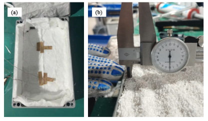
Assembly of insulation material: For Group A, the test material was placed around the heat source as shown in Figure 1, forming the experimental assembly to evaluate the thermal insulation performance of each material.

Download: Download full-size image

Figure 1. Installation of 6 mm insulation layers:(a) 6 mm asbestos insulation; (b) 6 mm aerogel particle insulation.

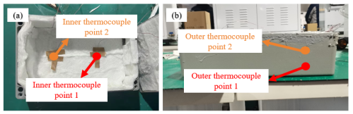
Experimental temperature measurement points: As shown in Figure 2, the temperature measurement points for Group A were arranged by placing thermocouples at paired inner and outer locations inside the container. Each inner temperature measurement point corresponded to a respective outer temperature measurement point, and the initial temperatures were recorded.

Download: Download full-size image

Figure 2. Temperature measurement points of 6 mm insulation layers: (a) 6 mm asbestos insulation; (b) 6 mm aerogel particle insulation.

Sealed Container: The container was sealed to ensure that heat transfer occurs primarily through the insulation material.

Temperature Recording: Temperatures inside and outside the container were recorded at regular time intervals to monitor thermal behavior.

Data Analysis: The temperature variations of different materials were compared to evaluate their thermal insulation performance. Analysis indicated that aerogel particles provided superior insulation, which was then selected for Group B experiments.

For Group B, experiments were conducted using a 10 mm thick aerogel particle insulation layer. The installation method and temperature measurement points were identical to those in Group A, with only the insulation thickness modified to obtain the corresponding thermal data.

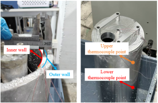
For Group C, the effect of drill collar thickness on the insulation layer was investigated. Drill collars of different wall thicknesses were used to simulate variations in structural thickness. The installation of a 10 mm drill collar insulation layer and the corresponding temperature measurement points are shown in Figure 3.

Download: Download full-size image

Figure 3. Installation and temperature measurement points of 10 mm aerogel particle insulation with 10 mm drill collar thickness.

The data from each experimental group were exported to Excel and plotted as line graphs to illustrate temperature variations over time.

2.3. Experimental Data Analysis

The following section presents the temperature variation data over time for each experimental group, obtained from the conducted tests. Temperatures were comprehensively recorded at multiple locations, including the outer high-temperature point, outer low-temperature point, inner high-temperature point, inner low-temperature point, and the hot oil temperature at different time intervals. The data obtained from the three experimental groups were subsequently analyzed to evaluate the thermal insulation performance of different materials, thicknesses, and drill collar structures.

2.3.1. Group A Data Analysis

The experimental data for Group A, using asbestos and aerogel particles both with a thickness of 6 mm, are presented in Figures 4 and 5.

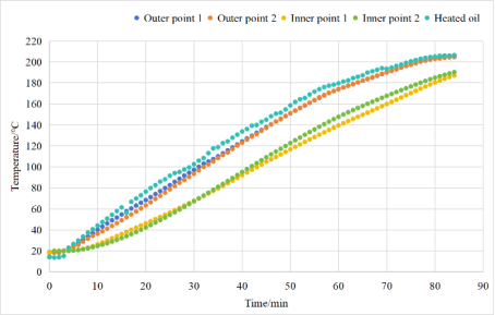
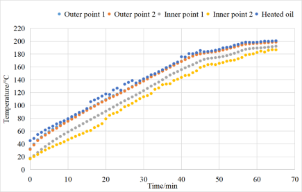
As shown in Figure 4, under 150°C hot oil conditions, the instantaneous temperature difference across the 6 mm aerogel particle insulation reached 31°C, with inner measurement point 1 and point 2 temperatures of 109°C and 114°C, respectively. At 175°C hot oil, the instantaneous temperature difference was 32°C, with inner point 1 and point 2 temperatures of 130°C and 138°C. At 200°C hot oil, the instantaneous temperature difference decreased to 24°C, with inner point 1 and point 2 temperatures of 170°C and 176°C.

Download: Download full-size image

Figure 4. Scatter plot of experimental data for 6 mm aerogel particle insulation.

As shown in Figure 5, for the 6 mm asbestos insulation under the same conditions, the instantaneous temperature difference reached 20°C at 150°C hot oil, with inner point 1 and point 2 temperatures of 132°C and 128°C. At 175°C hot oil, the instantaneous temperature difference was 17°C, with inner point 1 and point 2 temperatures of 151°C and 140°C. At 200°C hot oil, the instantaneous temperature difference decreased to 11°C, with inner point 1 and point 2 temperatures measured at 186°C and 159°C.

Download: Download full-size image

Figure 5. Scatter plot of experimental data for 6 mm asbestos insulation.

Temperature fluctuations observed in the hot oil curves were caused by bubble formation during heating, which led to variations in the measured values. From these results, it can be concluded that, at the same thickness, aerogel particles provide superior thermal insulation performance compared to asbestos.

2.3.2. Group B Data Analysis

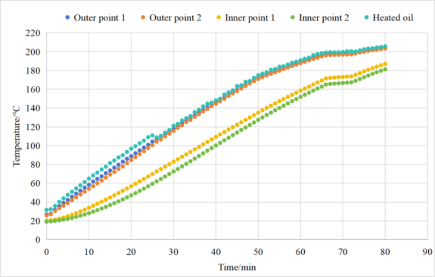
The experimental results for Group B, using a 10 mm aerogel particle insulation layer, are presented in Figure 6. Under 150°C hot oil conditions, the instantaneous temperature difference reached 42°C, with inner measurement point 1 and point 2 temperatures of 111°C and 102°C, respectively. At 175°C hot oil, the instantaneous temperature difference was 40°C, with inner point 1 and point 2 temperatures of 135°C and 127°C. At 200°C hot oil, the instantaneous temperature difference decreased to 31°C, with inner point 1 and point 2 temperatures of 173°C and 167°C. A comparison between Figures 4 and 6 indicates that, under the same external conditions, increasing the thickness of the aerogel particle insulation improves thermal insulation performance.

Download: Download full-size image

Figure 6. Scatter plot of experimental data for 10 mm aerogel particle insulation.

2.3.3. Group C Data Analysis

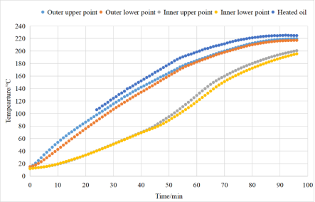
The experimental results for Group C, evaluating the effect of drill collar thickness on the insulation performance, are shown in Figure 7. Under 150°C hot oil conditions, the instantaneous temperature difference reached 70°C, with inner measurement point 1 and point 2 temperatures of 68°C and 67°C, respectively. At 175°C hot oil, the instantaneous temperature difference was 73°C, with inner point 1 and point 2 temperatures of 92°C and 86°C. At 200°C hot oil, the instantaneous temperature difference decreased to 60°C, with inner point 1 and point 2 temperatures of 132°C and 122°C.

These results demonstrate that the drill collar thickness significantly affects the thermal insulation performance of the insulation layer, with thicker drill collars enhancing the overall insulation effect.

Download: Download full-size image

Figure 7. Scatter plot of experimental data for 10 mm aerogel particle insulation with varying drill collar thickness.

2.3.4. Summary of Data Analysis

A systematic analysis of the experimental data from Groups A, B, and C revealed the effects of insulation material properties, material thickness, and drill collar structure on thermal insulation performance. The results indicate that aerogel particles exhibit significantly superior thermal insulation compared to asbestos. Under the same thickness and high-temperature conditions, the instantaneous temperature difference achieved by aerogel particles was up to 136% higher than that of asbestos. The low thermal conductivity of aerogel particles enables more effective thermal resistance under high-temperature conditions.

Regarding material thickness, the thermal insulation performance of aerogel particles was found to increase significantly with thickness. When the thickness was increased from 6 mm to 10 mm, the average instantaneous temperature difference across all tested temperature conditions increased by approximately 32%, demonstrating that a thicker insulation layer effectively extends the heat transfer path, reduces thermal conduction, and enhances overall insulation performance.

In addition, drill collar structure was shown to have an important influence on insulation performance. Data from Group C experiments indicate that, under the same material and thickness, increasing the drill collar thickness led to a maximum improvement of 87% in instantaneous temperature difference compared with Group B. This result demonstrates that tailored drill collar structures can affect insulation effectiveness and produce a synergistic effect with the insulation material, providing a new technical direction for optimizing thermal management systems.

These experimental findings provide quantitative guidance for selecting insulation materials and designing structural components for downhole MWD instruments. They confirm that aerogel particles, increased insulation thickness, and appropriately designed drill collar structures are effective strategies to enhance thermal insulation performance in high-temperature downhole environments.

3. Thermal Management Structure Design

3.1. Heat Generation Calculation

The downhole MWD instrument is represented by a Raman instrument for heat generation analysis. The relevant parameters are listed in Table 2.

Table 2. Parameters of the Raman Instrument.

Component	Parameters
Laser	75 mm (L) × 26 mm (W) × 80 mm (H)
Mainboard	127 mm (L) × 29 mm (W) × 57 mm (H)
Control Board	53 mm (L) × 13 mm (W) × 34 mm (H)
Vibration Frequency	100-150 Hz; Amplitude: 3 cm
Weight	< 3 kg

Download: Download full-size image

Figure 8. Structure of the Raman instrument within the protective enclosure.

The Raman instrument was placed inside a protective enclosure, as shown in Figure 8. To accommodate the instrument and the insulation layer, the dimensions of the enclosure were designed as follows: length 260 mm + 20 mm insulation thickness, width 30 mm + 20 mm, and height 80 mm + 20 mm. The resulting overall dimensions of the instrument enclosure are 280 mm (L) × 50 mm (W) × 100 mm (H).

3.1.1. Internal Instrument Heat Generation

The primary internal heat source of the instrument originates from the electrical energy consumed by the Raman spectrometer during operation. The heat generated can be calculated using the following relationship:

Q_{1} =P t θ

(1)

where

P

is the operating power of the Raman instrument,

t

is the unit operation time, and

θ

is the heat efficiency factor. Under typical working conditions, the Raman instrument generates approximately 720 J of internal heat per minute.

The corresponding temperature rise of the instrument due to internal heat generation can be evaluated using the specific heat relationship:

Q_{1} =m ∙ c ∙ {ΔT}_{1}

(2)

where

m

is the mass of the instrument,

c

is the specific heat capacity, and

Δ T_{1}

is the temperature rise. Based on the instrument mass and specific heat parameters, the internal heat causes a temperature increase of approximately 1.44°C per minute.

3.1.2. External Heat Conduction

The study objective of this study is to investigate the feasibility of the cooling system and evaluate its key performance parameters. To focus on the essential research goals and simplify the numerical simulation process without compromising computational accuracy, a steady-state heat transfer model is adopted in this work. Considering the actual geological conditions and the research focus on the cooling system’s performance, the formation is simplified as an external heat source. Based on relevant engineering practices and existing research on sandstone oil-bearing formations at a depth of 6000 m, the key thermophysical parameters of the formation are determined as follows: thermal conductivity λ = 3.0 W/(m·K), density ρ = 2500 kg/m³, and specific heat capacity c = 900 J/(kg·K). These parameter values are selected to ensure the reliability and rationality of the subsequent simulation analysis.

The primary external heat source is the high-temperature formation, which conducts heat to the instrument cavity through the drill collar and insulation layer. The heat transfer path consists of two stages: (1) heat conduction from the formation through the drill collar to the outer surface of the insulation layer, and (2) heat conduction through the insulation layer to the instrument.

The heat flux through the drill collar can be calculated using Fourier’s law of heat conduction:

P_{z} = λ ∙ A ∙ \frac{∆T}{δ}

(3)

where

λ

is the thermal conductivity of the drill collar,

A

is the contact area,

Δ T

is the temperature difference, and

δ

is the heat transfer path length. Under the selected working conditions, the drill collar transfers approximately 153.6 kJ per minute to the outer surface of the insulation layer. This heat results in a significant temperature rise at the drill collar, with a calculated increase of approximately 42.73°C per minute.

The heat then conducts through the insulation layer to the instrument. The corresponding heat flux is expressed as:

P_{g} =λ ∙ A ∙ \frac{∆T}{δ}

(4)

where

λ

is the thermal conductivity of the insulation layer, and other parameters are as defined previously. The heat transmitted through the insulation layer to the instrument is approximately 555.84 J per minute. Using the heat capacity relationship:

Q_{2} = P_{g} ∙ t ∙ θ

(5)

the contribution of external heat to the instrument temperature rise is approximately 0.93°C per minute.

3.2. TEC Cooling Efficiency Calculation

3.2.1. Basic Principle of TEC Cooling

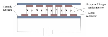
The Thermoelectric Cooler (TEC), also known as a thermoelectric module, is a heat dissipation device based on the Peltier effect (thermoelectric effect). It consists of a pair of P-type and N-type semiconductors. When an electric current passes through the module, electron-hole pairs are generated at one junction, absorbing heat and lowering the temperature to form the cold side, while at the other junction, recombination of electron-hole pairs releases heat, forming the hot side

[10]

A single P-N pair generates a limited temperature difference, but multiple pairs can be connected in series or parallel and encapsulated with ceramic plates to form a TEC device. One side serves as the cold face and the other as the hot face. Essentially, the TEC transfers heat from the cold side to the hot side. During this process, electrical current is supplied to the device, which also generates additional heat

[11-13]

TEC operation involves Joule heating, Fourier heat conduction, and the Thomson effect

[14]

. Since the Thomson effect is secondary and negligible under small operating currents and temperature differences, it is often ignored in engineering design. Material properties are typically assumed constant and evaluated at the average temperature of the cold and hot junctions

[15]

A typical TEC operating between a high-temperature source

T_{h}

and a low-temperature source

T_{c}

is shown in Figure 9. It consists of N-type and P-type semiconductor elements and a DC power supply. The TEC parameters include element lengths

L_{n}, L_{p}

, cross-sectional areas, thermal conductivities

k_{n}, k_{p}

, electrical conductivities

σ_{n}, σ_{p}

, Seebeck coefficients

S_{n}, S_{p}

, Thomson coefficients

τ_{n}, τ_{p}

, and the current

I

. The heat absorbed from the cold side and rejected to the hot side per unit time are denoted by

Q_{c}

and

Q_{h}

, respectively

[16]

Download: Download full-size image

Figure 9. Schematic diagram of the thermoelectric (TEC) device.

The thermoelectric semiconductor selected for this study is shown in Figure 10.

Download: Download full-size image

Figure 10. Photograph of the selected thermoelectric (TEC) semiconductor module.

The selected thermoelectric (TEC) module for this study has the following specifications and requirements:

The module resistance ranges from 2.062 to 2.519 Ω at an ambient temperature of 25°C.

The wire material is 20 AWG E-type Teflon, compliant with MIL-W-16878E/4.

The wire terminals are pre-tinned to ensure reliable electrical connections.

The cold side of the module is marked with the part number and batch number for identification.

The module complies with RoHS environmental standards.

Table 3. Basic Parameters of the Thermoelectric (TEC) Module.

Parameter	Value	Test Conditions
Maximum Current (I_max)	6.0 A	$Q_{c} = 0$ , $Δ T = Δ T_{max}$ , $T_{h} = 50$ °C
Maximum Voltage	18.3 V	$Q_{c} = 0$ , $I = I_{max}$ , $T_{h} = 50$ °C
Maximum Temperature	111°C	$Q_{c} = 0$ , $I = I_{max}$ , $T_{h} = 50$ °C
Maximum Heat Pumping Capacity	22 W	$I = I_{max}$ , $Δ T = 0$ , $T_{h} = 50$ °C
Maximum Instantaneous Temperature	200°C	Instantaneous measurement

3.2.2. TEC Cooling Capacity Calculation

To address the problem of heat accumulation in high-temperature downhole environments, a thermoelectric (TEC) cooling module was introduced, and a mathematical model of its heat absorption capacity was established for theoretical evaluation. The heat absorption power at the cold side of the TEC can be expressed as

[17]

P_{c} =α ∙ I ∙ ∆T - R ∙ I^{2}

(6)

where

P_{c}

is the cooling power (heat absorbed at the cold side),

α

is the Seebeck coefficient,

I

is the operating current,

Δ T

is the temperature difference between the cold and hot sides, and

R

is the internal resistance of the module. Under typical operating conditions (

Δ T = 160

°C,

I = 2.5

A), the cooling capacity of a single TEC element is approximately 26.6 W.

Considering heat transfer over a unit time of 60 s, the total heat absorbed by the TEC per minute can be expressed as:

Q_{3} = P_{c} ∙ t ∙ θ

(7)

where

t

is the operation time and

θ

is the heat transfer efficiency factor. The calculation shows that a single TEC element absorbs approximately 1277.5 J per minute.

The corresponding temperature decrease of the instrument can be estimated using the heat capacity relationship:

Q_{3} =m ∙ c ∙ {ΔT}_{3}

(8)

Assuming an instrument mass of 0.5 kg and a specific heat capacity of 1200 J/(kg·°C), the temperature reduction caused by a single TEC element is approximately 2.13°C per minute.

3.2.3. Temperature Rise Assessment

To comprehensively evaluate the temperature control capability, the thermal balance of the instrument was simulated under continuous operation for 100 hours:

Internal heat generation: the Raman instrument operates at 15 W with an efficiency factor of 0.8.

External heat conduction: formation heat transferred to the instrument through the drill collar and insulation layer.

Cooling by TEC: total heat absorbed by a single TEC element over the same time period.

The temperature change of the instrument due to net heat transfer can be estimated as:

ΔQ=m ∙ c ∙ ΔT

(9)

By combining the heat contributions, the net temperature rise can be calculated as:

ΔT = \frac{ΔQ}{mc} = \frac{Q_{1, total} + Q_{2,total} - Q_{3,total}}{mc}

(10)

Under these conditions, the cumulative temperature rise of the instrument after 100 hours of operation is approximately 33.34°C. Assuming an initial temperature of 20°C, the final temperature reaches 53.34°C, which exceeds the instrument’s temperature control limit of 50°C. To ensure the working temperature remains within safe limits, the design adopts two TEC elements, thereby significantly enhancing the cooling capacity and enabling stable operation of the instrument over prolonged periods. However, the extreme downhole environment featured with high pressure and intense vibration brings notable challenges to the long-term reliability of TECs, which is a key factor affecting the stable operation of the entire instrument system.

Specifically, high downhole static pressure is likely to induce deformation of TEC packaging and deterioration of internal thermocouple contact performance, while continuous high vibration can trigger fatigue failure of solder joints, peeling of thermal interface layers, and an increase in contact thermal resistance. These issues will further lead to poor heat transfer efficiency of TECs and gradual degradation of their working stability. Additionally, the long-term high-temperature environment in downholes will accelerate the grain coarsening of TEC thermoelectric materials, metal diffusion, and interface oxidation reactions, which sequentially result in gradual attenuation of cooling performance, a decrease in the coefficient of performance (COP), and a reduction in equivalent cooling capacity.

With the extension of operating time, the temperature difference bearing capacity of TECs will decrease. To maintain the target temperature control accuracy of the instrument, it is necessary to increase the operating current of TECs, which in turn increases power consumption and the heat load on the hot end, forming a positive feedback deterioration loop between TEC performance and power consumption. To solve these problems and ensure the long-term reliable operation of TECs under downhole conditions, the proposed design optimizes the TEC assembly structure: anti-vibration reinforcement measures are adopted to reduce the impact of vibration, high-pressure equalizing packaging is used to resist downhole high pressure, and low-stress thermal interface assembly is employed to improve heat transfer stability. Furthermore, a power consumption upper limit and a high-precision temperature closed-loop protection mechanism are established. Through derated operation and periodic performance compensation strategies, the TECs can maintain sufficient cooling capacity margin, avoid power consumption exceeding the limit, and ensure stable and reliable temperature control of the instrument’s core cavity throughout the entire downhole mission cycle.

3.3. Construction of the Thermal Management Structure

Based on the conclusions from the insulation experiments, combined with the internal heat generation of the Raman instrument, heat conduction through the drill collar, and the calculated TEC cooling capacity, a thermal management structure model was established using SOLIDWORKS.

3.3.1. Selection of Heat Sink Fins

Under the complex downhole conditions of high pressure and high flow velocity, the heat sink fins must not only possess excellent thermal conductivity but also sufficient structural strength to ensure stability and reliability throughout the drilling cycle, as summarized in Table 4.

To guarantee that the fins do not fail during their service life, shear strength and bending strength analyses are required. These analyses ensure that the selected fin material and geometry can withstand operational stresses while maintaining efficient heat dissipation.

Table 4. Basic Parameters for Heat Sink Fin Design.

Parameter	Value
Downhole drilling fluid flow rate ( $Q$ )	40 L/s
Downstream drilling fluid pressure at sensor ( $P_{1}$ )	70 MPa

Shear Strength Analysis: Under high-velocity drilling fluid flow, the heat sink fins are subjected to significant shear loads. The shear stress can be calculated as:

τ_{s} = \frac{F}{A_{s}}

(11)

where

F

is the force exerted by the downward drilling fluid on the fin surface, and

A_{s}

is the area of the fin subjected to the load. Based on known drilling fluid parameters such as density, flow rate, and velocity, the shear force was calculated using the principle of momentum conservation, and the actual shear stress on the fin was determined from the cross-sectional area.

The calculation indicates that the actual shear stress of the fin is 73 MPa, which is well below the allowable shear stress of commonly used metals such as aluminum alloys or titanium alloys. Therefore, the structural design meets safety requirements.

Bending Strength Analysis: The heat sink fins also experience bending moments due to drilling fluid impact. The bending stress can be calculated as:

σ_{s} = \frac{M_{s}}{W}

(12)

where

M_{s}

is the bending moment at the fin root induced by the impact load, and

W

is the section modulus of the fin.

By substituting the structural parameters into the formula, the maximum bending stress of the fin was calculated to be 39.42 MPa, the section modulus

W

is 833.33 mm³, and the bending moment

M_{s}

is 591.3 N·m. These results were used to select suitable materials for manufacturing the fins.

Based on material research, appropriate materials for the heat sink fins were selected, as summarized in Table 5.

Table 5. Analysis of Heat Sink Fin Materials.

Material	Thermoelectric / Thermal Performance	Mechanical Properties	Thermal Stability
Bismuth telluride and alloys	High thermoelectric figure of merit near room temperature	Brittle, relatively low mechanical strength	Good thermal stability within a certain temperature range; performance may degrade at high temperatures
Silicon-germanium alloy	Good thermoelectric performance at medium to high temperatures; thermoelectric figure of merit increases with temperature	Good mechanical strength and toughness, can withstand external force and thermal stress	Stable performance over a wide temperature range
Silicon carbide (SiC)	High thermal conductivity, enabling rapid heat transfer and improved heat dissipation efficiency	Excellent mechanical properties; high hardness and strength, can withstand high temperature and pressure without deformation	Excellent thermal stability; maintains physical and chemical properties at high temperatures; strong oxidation resistance
Copper	High thermal conductivity, efficiently transferring heat from the semiconductor device; excellent electrical conductivity	Good ductility and malleability; high hardness and strength; allows high machining precision and surface quality	Good ductility and malleability; high hardness and strength; allows high machining precision and surface quality

Based on the analysis of material properties, copper was selected as the fin material due to its excellent mechanical performance, high hardness, and strength, allowing it to withstand high-temperature and high-pressure downhole environments. A 3D model of the copper heat sink fins was constructed using SOLIDWORKS, as shown in Figure 11.

Download: Download full-size image

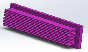
Figure 11. 3D model of the copper heat sink fins.

The fin parameters are as follows: total length 270 mm, base thickness 10.7 mm, single fin thickness 2 mm, single fin length 30 mm, and fin spacing 3 mm.

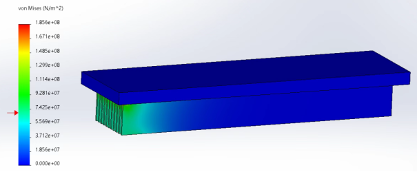
Figure 12 shows the stress simulation of the copper fins under impact from the downward-flowing drilling fluid. The front end maintains its shape under fluid impact, demonstrating that the copper material provides sufficient structural strength for the fin design. Most areas of the copper fins are colored blue, indicating relatively low stress levels within the safe range. Only the front-end region shows higher stress values (green), but these do not reach the material yield strength. This confirms that the copper fins can maintain structural integrity under the impact of downward drilling fluid without plastic deformation or failure.

Download: Download full-size image

Figure 12. Stress simulation of copper heat sink fins under downward drilling fluid impact.

3.3.2. Construction of the Thermal Management Structure Model

Based on the calculation data and design requirements described above, a 3D thermal management structure model was established using SOLIDWORKS, as shown in Figure 13.

Download: Download full-size image

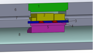
Figure 13. Cross-sectional view of the thermal management structure model.

In Figure 13:

Instrument chamber cover plate - serves as the enclosure of the instrument cavity, protecting internal components from intrusion of downhole drilling fluid and debris, while partially contributing to thermal insulation and conduction control.

Raman instrument - the key measurement device in the downhole MWD system; generates heat during operation and is a primary heat source that the cooling system must manage. Stable operation requires strict temperature control.

Heat sink plate - possesses high thermal capacity and mainly functions to secure the fins, stabilizing the overall heat dissipation structure.

Three-stage thermoelectric (TEC) modules - exploit the Peltier effect to actively pump heat from the cold side to the hot side. They play a critical role in reducing the internal temperature of the instrument and addressing high-temperature challenges.

Copper fins - made of high thermal conductivity copper, designed to increase the heat transfer surface area. They enhance convective heat transfer with the downward-flowing drilling fluid.

Drill collar (Ø203 mm) - serves as the mechanical support and protective structure for the instrument. Its material and geometry also influence heat transfer and distribution, participating in the overall thermal exchange process.

Cable passage - allows routing of internal wiring to ensure electrical connectivity between instrument components.

Downward drilling fluid channel - provides the convective medium for the copper fins. Circulating drilling fluid removes heat from the fins and is a key pathway for heat dissipation in the thermal management system.

4. Numerical Simulation

4.1. Thermal Management Structure Model

4.1.1. Geometric Model Simplification

Geometric simplification is a necessary step when performing numerical simulations of the downhole MWD instrument’s thermal management structure

[18]

. The actual instrument structure is highly complex, containing numerous components. Including all details in the model would significantly increase computational cost and simulation difficulty.

During simplification, emphasis is placed on the elements that critically affect heat dissipation, while features with minor impact are omitted. For example, small mounting holes and grooves on the instrument housing have negligible influence on overall thermal performance and are therefore ignored in the model. For components made of uniform metallic materials, removing fine features effectively reduces model complexity.

The Raman instrument, as the main heat source, is represented as an equivalent heat source that accounts for its total heat generation and spatial location. This approach significantly reduces model complexity and computational cost while ensuring that simulation results remain within an acceptable accuracy range.

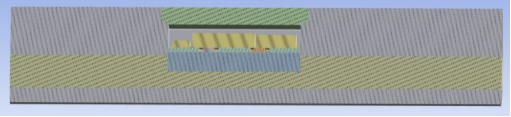
These simplification measures enable efficient numerical simulation and provide reliable guidance for optimizing the thermal management structure. Figure 14 shows the simplified geometric model used for the simulation.

Download: Download full-size image

Figure 14. Simplified geometric model of the thermal management structure.

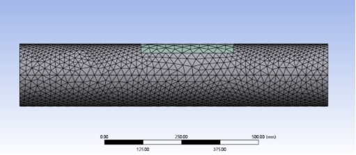
4.1.2. Mesh Generation

A reasonable mesh is critical for ensuring the accuracy of numerical simulations. For the simplified thermal management structure, an unstructured mesh was employed. Mesh refinement was applied in key regions, such as the contact areas between the heat-generating elements and the housing, and the surfaces where the downward-flowing drilling fluid interacts with the housing for convective heat transfer.

Local mesh refinement allows for more accurate capture of temperature gradients and heat flux in these critical areas. In regions far from the heat source where temperature changes are relatively gradual, the mesh size was increased appropriately to reduce the total number of cells and improve computational efficiency.

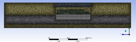
During meshing, the quality of the mesh was carefully checked to ensure parameters such as skewness and aspect ratio were within acceptable ranges, avoiding inaccurate results or convergence issues. The meshing process in ANSYS Fluent is illustrated in Figures 15 and 16.

Download: Download full-size image

Figure 15. Mesh generation of the thermal management structure.

Download: Download full-size image

Figure 16. Cross-sectional view of the mesh distribution.

4.2. Numerical Simulation Parameter Settings

4.2.1. Material Properties

Accurate material property definitions are essential for numerical simulation. For the housing of the logging-while-drilling instrument, aluminum alloy is adopted, with a thermal conductivity of 150 W/(m·K), a density of 2700 kg/m³, and a specific heat capacity of 850 J/(kg·K). The thermal conductivity of internal electronic components (e.g., chips) is set to 3 W/(m·K). Water-based drilling fluid is used as the downward-flowing fluid, which has a thermal conductivity of 0.55 W/(m·K), a density of 1100 kg/m³, and a specific heat capacity of 3500 J/(kg·K).

4.2.2. Boundary Conditions

The choice of boundary conditions directly affects the simulation outcomes. For the thermal management structure of the downhole instrument, the heat generation of internal electronic components is applied as an internal heat source boundary condition, based on measured data or component specifications. For example, if a component has a rated power of 5 W, this value is used as the heat input in the simulation.

For the housing surfaces in contact with the drilling fluid, convective heat transfer boundary conditions are applied. The convective heat transfer coefficient is determined based on drilling fluid velocity, temperature, and housing surface roughness, using empirical correlations or experimental data. For high drilling fluid flow rates, the convective heat transfer coefficient may range from 100 to 500 W/(m²·K).

Additionally, environmental temperature is specified as the far-field boundary condition. Downhole formation temperatures vary with depth, and the boundary temperature distribution is set according to measured formation temperature profiles.

4.3. Simulation Results Analysis

4.3.1. Temperature Field Distribution

The numerical simulation results reveal the temperature distribution of the downhole MWD instrument under various operating conditions. The simulations clearly illustrate the temperature profiles of internal components and the temporal evolution of temperatures. After a period of normal operation, high-temperature zones develop around the heat-generating elements, forming localized temperature peaks, with heat gradually dissipating to surrounding components and the housing.

The center temperature of the heat-generating chip can reach 120°C, decreasing progressively with distance from the chip. At the instrument housing surface, the temperature approaches that of the circulating drilling fluid. Analysis of the temperature field enables identification of high-temperature regions within the thermal management structure, providing guidance for subsequent structural optimization.

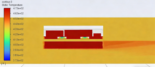
4.3.2. Heat Flux Density Analysis

Heat flux density analysis provides insight into the pathways and intensity of heat transfer within the thermal management structure. As illustrated in Figures 17 and 18, heat is primarily transferred from the Raman instrument to the copper fins via the thermoelectric (TEC) modules, and subsequently dissipated into the downward-flowing drilling fluid through convective heat transfer.

Regions where heat-generating elements contact the housing exhibit higher heat flux densities, indicating these areas are critical for heat transfer. By analyzing these results, the influence of the thermal management structure design on heat transfer efficiency can be evaluated. The color gradient, ranging from blue to red, represents low to high temperatures, respectively, confirming that drilling fluid flowing across the fins effectively removes heat, validating the rationality of the designed thermal management system.

Download: Download full-size image

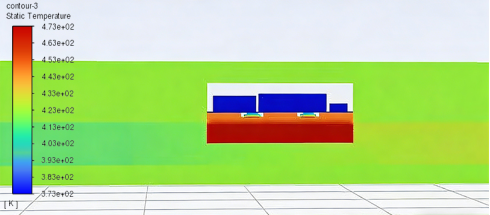
Figure 17. Longitudinal temperature contour (Case A - TEC inactive).

In Figure 17, the TEC modules were not activated, highlighting the contribution of drilling fluid convection in removing heat from the copper fins.

Download: Download full-size image

Figure 18. Longitudinal temperature contour (Case B - TEC active).

In Figure 18, TEC modules were activated, enabling active cooling of the Raman instrument. Comparison of Figures 17 and 18 demonstrates that TEC-based active cooling is highly effective, substantially absorbing the heat generated by the Raman instrument and reducing the heat transmitted to the fins.

4.3.3. Summary of Simulation Results

The simulation results confirm that the proposed thermal management design is effective in dissipating the heat generated by the instrument. To validate the reliability of the thermal model, analytical temperature rise calculations are compared with the numerical simulation results. The predicted temperature trends from theoretical analysis agree well with the simulation outputs, with minor deviations within an acceptable range, which supports the accuracy of the established model. Comparison of longitudinal temperature contours with and without TEC cooling shows that the TEC active cooling technology significantly reduces the internal temperature of the Raman instrument, while convective heat removal by the downward-flowing drilling fluid further enhances heat dissipation.

These results indicate that the improved thermal management structure optimizes heat transfer efficiency, lowers internal temperatures, and ensures stable operation of the downhole MWD instrument under high-temperature conditions.

5. Conclusions

A high-temperature-adaptive thermal management scheme for downhole MWD instruments was developed, and the following conclusions were drawn:

Influence of insulation materials, thickness, and drill collar structure:

Systematic analysis of the experimental data from Groups A, B, and C revealed the influence mechanisms of insulation material properties, material thickness, and drill collar structure on thermal performance. Group A demonstrated the decisive role of material properties on thermal insulation performance; Group B showed a positive correlation between material thickness and insulation effectiveness; and Group C highlighted the synergistic enhancement effect between drill collar structure and insulation material.

Synergistic TEC-copper fin design:

The combination of a three-stage thermoelectric cooler (TEC) and copper fins was validated through strength analysis and numerical simulation. Results show that the instrument housing temperature approaches the drilling fluid temperature, and heat flux is efficiently transferred along the designated path. This synergy forms a complete thermal management chain of “active cooling - high-efficiency conduction - convective heat dissipation”, effectively mitigating heat accumulation within the instrument and providing critical technical support for stable operation in high-temperature downhole environments.

Validation of optimized thermal management design:

Numerical simulations confirmed the effectiveness of the aerogel insulation combined with optimized drill collar structure, as well as the TEC + copper fin design. The TEC active cooling system significantly absorbs the heat generated by the Raman instrument, reducing the heat transmitted to the fins. Meanwhile, the convective effect of the downward-flowing drilling fluid further removes heat from the fins, providing a practical solution for downhole instrument thermal management.

Abbreviations

MWD	Measurement While Drilling
TEC	Thermoelectric Cooler

Author Contributions

Chengchi Wang: Conceptualization, Data curation, Formal analysis, Writing – original draft, Writing – review & editing

Yawen Jing: Software, Validation, Writing – original draft

Dongrui Su: Data curation, Formal analysis, Writing – original draft

Conflicts of Interest

The authors declare that they have no known competing financial interests or personal relationships that could have appeared to influence the work reported in this paper.

References

[1]	Su, Y., Lu, B., Liu, Y., et al. (2020). Current situation and research suggestions for drilling and completion technology of deep and ultra deep wells on land in China. Petroleum Drilling and Production Technology, 42(05), 527-542. https://doi.org/10.13639/j.odpt.2020.05.001
[2]	Zhao, J. (2022). Adaptability analysis of ultra deep well measurement instruments while drilling. China Petroleum and Chemical Industry Standards and Quality, 42(15), 95-97.
[3]	Ma, Q. (2016). Overview of drilling fluid cooling technology and equipment. Petroleum Machinery, 44(10), 42-46. https://doi.org/10.16082/j.cnki.issn.1001-4578.2016.10.010
[4]	Jiale, P., Wei, L., Fulong, W., et al. (2023). A numerical model coupling multiple heat transfer modes to develop a passive thermal management system for logging tool. Applied Thermal Engineering, 223. https://doi.org/10.1016/J.APPLTHERMALENG.2023.120011
[5]	Bennett, G. A. (1986). Active cooling for downhole instrumentation: Design criteria and conceptual design summary (LA-10723-MS) [Report]. Los Alamos: Los Alamos National Laboratory. https://www.osti.gov/biblio/5073612
[6]	Bennett, G. A. (1988). Active cooling for downhole instrumentation: Preliminary analysis and system selection (LA-1102-MS) [Report]. Santa Fe: Los Alamos National Laboratory. https://www.osti.gov/biblio/5360643
[7]	Bennett, G. A. (1991). Active cooling for downhole instrumentation: Miniature thermoacoustic refrigerator [Doctoral dissertation]. The University of New Mexico, Albuquerque, USA. https://digitalrepository.unm.edu/etds/UNM
[8]	Liu, K., Gao, W., Hong, D., et al. (2020). Research on the thermal resistance performance of downhole cooling system for drilling instruments. Petroleum Machinery, 48(08), 23-30. https://doi.org/10.16082/j.cnki.issn.1001-4578.2020.08.004
[9]	Liu, K., Su, Y., Gao, W., et al. (2022). Numerical study on cooling effect of downhole cooling system for drilling instruments. Petroleum Machinery, 50(07), 18-25+33. https://doi.org/10.16082/j.cnki.issn.1001-4578.2022.07.003
[10]	Wang, H. (2024). Development of a large dynamic high spatial resolution OTDR system [Doctoral dissertation]. University of Electronic Science and Technology of China. https://doi.org/10.27005/d.cnki.gdzku.2024.000825
[11]	Zhang, C. (2022). Optimization design and characteristics study of high temperature semiconductor thermoelectric refrigerator [Doctoral dissertation]. Nanjing University of Science and Technology. https://doi.org/10.27241/d.cnki.gnjgu.2022.001154
[12]	Yuan, Y., Yang, H., Zhang, S., et al. (2024). Discussion on current chip heat dissipation technology methods and characteristics. Science and Technology Vision, 14(21), 37-39.
[13]	Ding, S., Li, S., Hu, M., et al. (2025). Design and implementation of intelligent temperature reduction clothing based on semiconductor refrigeration chips. Modern Information Technology, 9(06), 5-9. https://doi.org/10.19850/j.cnki.2096-4706.2025.06.002
[14]	Peng, Q. (2019). Development analysis of semiconductor refrigeration technology. Integrated Circuit Applications, 36(07), 94-95. https://doi.org/10.19339/j.issn.1674-2583.2019.07.038
[15]	Li, Y. (2007). Optimization design of semiconductor multi-stage refrigeration performance combination [Doctoral dissertation]. Tongji University.
[16]	Dang, C. (2012). Experimental study on integrated constant temperature heat sink based on semiconductor cooler TEC [Doctoral dissertation]. Jilin University.
[17]	Liu, X., Ma, X. (2021). Research on semiconductor refrigeration technology and application path. Information Recording Materials, 22(04), 131-132. https://doi.org/10.16009/j.cnki.cn13-1295/tq.2021.04.076
[18]	Xue, Z., Shang, B., Zhang, J., et al. (2021). Numerical simulation analysis of thermal management system for high-temperature downhole logging tool. Drilling and Production Technology, 44(05), 92-96.

Cite This Article

Plain Text BibTeX RIS

APA Style

Wang, C., Jing, Y., Su, D., Yu, G., Lin, Z. (2026). Research on a Thermal Management System for Downhole Measurement-While-Drilling Instruments. Modern Chemistry, 14(1), 22-37. https://doi.org/10.11648/j.mc.20261401.13

Copy | Download

ACS Style

Wang, C.; Jing, Y.; Su, D.; Yu, G.; Lin, Z. Research on a Thermal Management System for Downhole Measurement-While-Drilling Instruments. Mod. Chem. 2026, 14(1), 22-37. doi: 10.11648/j.mc.20261401.13

Copy | Download

AMA Style

Wang C, Jing Y, Su D, Yu G, Lin Z. Research on a Thermal Management System for Downhole Measurement-While-Drilling Instruments. Mod Chem. 2026;14(1):22-37. doi: 10.11648/j.mc.20261401.13

Copy | Download

@article{10.11648/j.mc.20261401.13,
  author = {Chengchi Wang and Yawen Jing and Dongrui Su and Guixin Yu and Zejing Lin},
  title = {Research on a Thermal Management System for Downhole Measurement-While-Drilling Instruments},
  journal = {Modern Chemistry},
  volume = {14},
  number = {1},
  pages = {22-37},
  doi = {10.11648/j.mc.20261401.13},
  url = {https://doi.org/10.11648/j.mc.20261401.13},
  eprint = {https://article.sciencepublishinggroup.com/pdf/10.11648.j.mc.20261401.13},
  abstract = {As oil and gas exploration extends toward deep and ultra-deep formations, downhole measurement-while-drilling (MWD) instruments are subjected to increasingly severe high-temperature environments, making efficient thermal management essential for stable operation. This study presents the engineering design of a thermal management system for downhole MWD instruments. Thermal insulation material selection, heat dissipation structure design, and numerical simulation are combined to develop a system suitable for high-temperature downhole conditions. A comparative evaluation of asbestos and aerogel particle insulation demonstrates that the insulation temperature difference increases with aerogel thickness, indicating a strong dependence of thermal insulation performance on material thickness. The thickness of the drill collar structure is also shown to influence overall insulation effectiveness. Considering the heat generation of the Raman instrument and external heat conduction, a heat dissipation structure integrating three-stage thermoelectric cooler (TEC) active cooling with copper fin-enhanced convective heat transfer is proposed. Key geometric parameters of the copper fins are determined based on TEC cooling capacity and structural strength requirements. A three-dimensional thermal model including the heat sink plate and drill collar is established and analyzed using ANSYS Fluent. Simulation results indicate that the tool housing temperature approaches the drilling fluid temperature after TEC cooling and fin-assisted heat dissipation. Heat flux analysis confirms efficient heat transfer along the “TEC-copper fins-drilling fluid” pathway. The proposed synergistic thermal management design provides effective engineering support for downhole MWD instruments operating in high-temperature environments.},
 year = {2026}
}

Copy | Download

TY  - JOUR
T1  - Research on a Thermal Management System for Downhole Measurement-While-Drilling Instruments
AU  - Chengchi Wang
AU  - Yawen Jing
AU  - Dongrui Su
AU  - Guixin Yu
AU  - Zejing Lin
Y1  - 2026/02/27
PY  - 2026
N1  - https://doi.org/10.11648/j.mc.20261401.13
DO  - 10.11648/j.mc.20261401.13
T2  - Modern Chemistry
JF  - Modern Chemistry
JO  - Modern Chemistry
SP  - 22
EP  - 37
PB  - Science Publishing Group
SN  - 2329-180X
UR  - https://doi.org/10.11648/j.mc.20261401.13
AB  - As oil and gas exploration extends toward deep and ultra-deep formations, downhole measurement-while-drilling (MWD) instruments are subjected to increasingly severe high-temperature environments, making efficient thermal management essential for stable operation. This study presents the engineering design of a thermal management system for downhole MWD instruments. Thermal insulation material selection, heat dissipation structure design, and numerical simulation are combined to develop a system suitable for high-temperature downhole conditions. A comparative evaluation of asbestos and aerogel particle insulation demonstrates that the insulation temperature difference increases with aerogel thickness, indicating a strong dependence of thermal insulation performance on material thickness. The thickness of the drill collar structure is also shown to influence overall insulation effectiveness. Considering the heat generation of the Raman instrument and external heat conduction, a heat dissipation structure integrating three-stage thermoelectric cooler (TEC) active cooling with copper fin-enhanced convective heat transfer is proposed. Key geometric parameters of the copper fins are determined based on TEC cooling capacity and structural strength requirements. A three-dimensional thermal model including the heat sink plate and drill collar is established and analyzed using ANSYS Fluent. Simulation results indicate that the tool housing temperature approaches the drilling fluid temperature after TEC cooling and fin-assisted heat dissipation. Heat flux analysis confirms efficient heat transfer along the “TEC-copper fins-drilling fluid” pathway. The proposed synergistic thermal management design provides effective engineering support for downhole MWD instruments operating in high-temperature environments.
VL  - 14
IS  - 1
ER  -

Copy | Download

Author Information

Chengchi Wang

College of Petroleum Engineering, Liaoning Petrochemical University, Fushun, China

Contact Email
Yawen Jing

School of Art and Design, Liaoning Petrochemical University, Fushun, China

Contact Email
Dongrui Su

College of Petroleum Engineering, Liaoning Petrochemical University, Fushun, China

Contact Email
Guixin Yu

College of Petroleum Engineering, Liaoning Petrochemical University, Fushun, China
Zejing Lin

College of Petroleum Engineering, Liaoning Petrochemical University, Fushun, China

Download PDF

Submit an Article

Plain Text BibTeX RIS

APA Style

Wang, C., Jing, Y., Su, D., Yu, G., Lin, Z. (2026). Research on a Thermal Management System for Downhole Measurement-While-Drilling Instruments. Modern Chemistry, 14(1), 22-37. https://doi.org/10.11648/j.mc.20261401.13

Copy | Download

ACS Style

Wang, C.; Jing, Y.; Su, D.; Yu, G.; Lin, Z. Research on a Thermal Management System for Downhole Measurement-While-Drilling Instruments. Mod. Chem. 2026, 14(1), 22-37. doi: 10.11648/j.mc.20261401.13

Copy | Download

AMA Style

Wang C, Jing Y, Su D, Yu G, Lin Z. Research on a Thermal Management System for Downhole Measurement-While-Drilling Instruments. Mod Chem. 2026;14(1):22-37. doi: 10.11648/j.mc.20261401.13

Copy | Download

@article{10.11648/j.mc.20261401.13,
  author = {Chengchi Wang and Yawen Jing and Dongrui Su and Guixin Yu and Zejing Lin},
  title = {Research on a Thermal Management System for Downhole Measurement-While-Drilling Instruments},
  journal = {Modern Chemistry},
  volume = {14},
  number = {1},
  pages = {22-37},
  doi = {10.11648/j.mc.20261401.13},
  url = {https://doi.org/10.11648/j.mc.20261401.13},
  eprint = {https://article.sciencepublishinggroup.com/pdf/10.11648.j.mc.20261401.13},
  abstract = {As oil and gas exploration extends toward deep and ultra-deep formations, downhole measurement-while-drilling (MWD) instruments are subjected to increasingly severe high-temperature environments, making efficient thermal management essential for stable operation. This study presents the engineering design of a thermal management system for downhole MWD instruments. Thermal insulation material selection, heat dissipation structure design, and numerical simulation are combined to develop a system suitable for high-temperature downhole conditions. A comparative evaluation of asbestos and aerogel particle insulation demonstrates that the insulation temperature difference increases with aerogel thickness, indicating a strong dependence of thermal insulation performance on material thickness. The thickness of the drill collar structure is also shown to influence overall insulation effectiveness. Considering the heat generation of the Raman instrument and external heat conduction, a heat dissipation structure integrating three-stage thermoelectric cooler (TEC) active cooling with copper fin-enhanced convective heat transfer is proposed. Key geometric parameters of the copper fins are determined based on TEC cooling capacity and structural strength requirements. A three-dimensional thermal model including the heat sink plate and drill collar is established and analyzed using ANSYS Fluent. Simulation results indicate that the tool housing temperature approaches the drilling fluid temperature after TEC cooling and fin-assisted heat dissipation. Heat flux analysis confirms efficient heat transfer along the “TEC-copper fins-drilling fluid” pathway. The proposed synergistic thermal management design provides effective engineering support for downhole MWD instruments operating in high-temperature environments.},
 year = {2026}
}

Copy | Download

TY  - JOUR
T1  - Research on a Thermal Management System for Downhole Measurement-While-Drilling Instruments
AU  - Chengchi Wang
AU  - Yawen Jing
AU  - Dongrui Su
AU  - Guixin Yu
AU  - Zejing Lin
Y1  - 2026/02/27
PY  - 2026
N1  - https://doi.org/10.11648/j.mc.20261401.13
DO  - 10.11648/j.mc.20261401.13
T2  - Modern Chemistry
JF  - Modern Chemistry
JO  - Modern Chemistry
SP  - 22
EP  - 37
PB  - Science Publishing Group
SN  - 2329-180X
UR  - https://doi.org/10.11648/j.mc.20261401.13
AB  - As oil and gas exploration extends toward deep and ultra-deep formations, downhole measurement-while-drilling (MWD) instruments are subjected to increasingly severe high-temperature environments, making efficient thermal management essential for stable operation. This study presents the engineering design of a thermal management system for downhole MWD instruments. Thermal insulation material selection, heat dissipation structure design, and numerical simulation are combined to develop a system suitable for high-temperature downhole conditions. A comparative evaluation of asbestos and aerogel particle insulation demonstrates that the insulation temperature difference increases with aerogel thickness, indicating a strong dependence of thermal insulation performance on material thickness. The thickness of the drill collar structure is also shown to influence overall insulation effectiveness. Considering the heat generation of the Raman instrument and external heat conduction, a heat dissipation structure integrating three-stage thermoelectric cooler (TEC) active cooling with copper fin-enhanced convective heat transfer is proposed. Key geometric parameters of the copper fins are determined based on TEC cooling capacity and structural strength requirements. A three-dimensional thermal model including the heat sink plate and drill collar is established and analyzed using ANSYS Fluent. Simulation results indicate that the tool housing temperature approaches the drilling fluid temperature after TEC cooling and fin-assisted heat dissipation. Heat flux analysis confirms efficient heat transfer along the “TEC-copper fins-drilling fluid” pathway. The proposed synergistic thermal management design provides effective engineering support for downhole MWD instruments operating in high-temperature environments.
VL  - 14
IS  - 1
ER  -

Copy | Download