1. Introduction
Modelling dependence among non-normal random variables has become increasingly important in modern statistical and applied research, largely because real-world datasets often violate the normality assumption. Multivariate Gaussian models are often inadequate when variables exhibit heavy tails, asymmetries, or nonlinear dependencies. Copula methods, which separate marginal behavior from joint dependence, offer a flexible framework for constructing valid joint distributions even when marginal distributions are non-Gaussian
.
The modern appeal to copulas stems from the work of Embrechts et al.
| [3] | P. Embrechts, A. McNeil & D. Straumann, Correlation and dependence in risk management: Properties and pitfalls. In M. Dempster (Ed.), Risk management: Value at risk and beyond, 1999), pp. 176-223. Cambridge University Press.
https://doi.org/10.1017/CBO9780511615337.008 |
[3]
, whose seminal exposition showed how to model non-normal dependence via copula theory. As a result, copula models have rapidly gained traction across many fields. In finance, directional dependence in foreign exchange markets has been studied using copulas
, and copulas have been used in pricing collateralized debt obligations
. In hydrology and climatology, copulas have enabled multivariate drought assessment
| [6] | C. de Michele, G. Salvadori, R. Vezzoli, & S. Pecora, Multivariate assessment of droughts: Copula-based analysis of severity and duration. Water Resources Research, 2013, 49(10), 6985 - 6994, https://doi.org/10.1002/wrcr.20548 |
[6]
. In genomics, they have been used to capture dependence structures between genes
. And in reliability and engineering, copulas have been applied to model dependence in wind speeds or other system components
. Recently, dependence among anthropometric variables were also modeled using copulas
| [9] | F. W. O. Saporu & I. E. Gongsin, “Modelling Dependence Relationships of Anthropometric Variables Using Copula Approach”, American Journal of Theoretical and Applied Statistics, 2020, Vol. 9, No. 5, pp. 245 - 255,
https://doi.org:10.11648/j.ajtas.20200905.18 |
[9]
.
In recent literature, many further developments in copula theory and applications have been witnessed. For example, large skew-t copula models have been proposed to capture asymmetric and heavy-tail dependence in financial time series
| [10] | L. Deng, M. S. Smith & W. Maneesoonthon, “Large skew-t copula models and Asymmetric Dependence in intraday Equity Returns”, Journal of Business & Economic Statistics, 43(2) 269 - 285, (2025) https://doi.org/10.1080/07350015.2024.2360592 |
[10]
. New reviews highlight evolving trends such as vine copula simplification, factor copulas, and applications in censored survival settings
| [11] | O. Crommen, P. Janssen & N. Veraverbeke, “Vine copula simplification: A comprehensive review”, SORT, 2025, 49(1), 67 - 102, https://raco.cat/index.php/SORT/article/view/433164 |
| [12] | A. I. N. Miguel, “A Comprehensive Review of Copulas in Multivariate Dependency Modelling”, (September 09, 2024). Available at SSRN: https://dx.doi.org/10.2139/ssrn.4950425 |
[11, 12]
. Copula-based joint regression frameworks and survival models are receiving more attention, especially for non-normal correlated outcomes
.
Beyond copulas, the literature also contains direct methods for constructing multivariate non-normal distributions. Early expositions include Ref.s
| [14] | S. Kotz, N. Balakrishnan & N. L. Johnson, Continuous multivariate distributions, (2000). Volume 1: Models and applications (2nd ed.). Wiley. https://doi.org/10.1002/0471722065 |
| [15] | J. M. Sarabia & G. Emilio, “Construction of multivariate distributions with given marginal and correlation matrix”, Journal of Multivariate Analysis, 99(6) (2008), 1262 - 1275.
https://doi.org/10.1016/j.jmva.2007.07.005 |
| [16] | N. Balakrishnan, & C. D. Lai, Continuous bivariate distributions (2nd ed.), 2009. Springer.
https://doi.org/10.1007/b101765 |
[14-16]
. These approaches generally specify joint densities or cumulative functions in closed form, often by extending univariate distributions or using conditioning constructs. In the conditional approach, one builds a bivariate (or multivariate) distribution by specifying a marginal and then a conditional distribution. For example, Gongsin & Saporu
developed a bivariate conditional Weibull model, and Sens et al.
| [18] | S. Sens, R Lamichhane & N. Diawara, “A Bivariate Distribution with Conditional Gamma and its Multivariate Form”, Journal of Modern Applied Statistical Methods, vol. 13, No 2 Article 9, 169 - 184. 2014,
https://doi.org/10.22237/jmasm/1414814880 |
[18]
proposed a bivariate distribution combining conditional gamma constructs. Another path uses the probability integral transform, for example, Ref.
| [19] | D. Villanueva, A. Feijoo & J. L.Pazos, “Multivariate Weibull Distribution for Wind Speed and Wind Power Behavior Assessment”, Resources, 2013, 2, 370 - 384,
https://doi.org:10.3390/resources2030370 |
[19]
constructed multivariate Weibull distribution by mapping the Weibull variables into standard normal variables for wind speed and wind power modelling. In Ref.
the power law transformations of vector components with Gaussian, isotropic, mean-zero variability, was used to construct a bivariate distribution for modelling wind speed from different altitudes.
Nevertheless, many of the existing constructions are limited in flexibility, that is, they may only produce simple hazard shapes, or be difficult to generalize. In environmental and reliability contexts, where variables like wind speed often exhibit complex dependence and nonlinear tails, richer multivariate models are needed. Indeed, recent joint modelling of wind and waves, or wind and other environmental covariates, relies heavily on vine copula frameworks, see for example,
| [21] | J. Wu, X. Li & T. Zhou, “Copula-based joint modelling of wind and wave parameters for marine engineering” Journal of Marine Science and Engineering, 2025, 13(3), 396.
https://doi.org/10.3390/jmse13030396 |
[21]
. The Clayton copula was used to model the joint distribution of extreme wind speed and air density for structural wind load assessment
. However, which bivariate model to use for a given situation is not generally known a priori and is usually determined empirically through statistical model selection criteria.
In light of these developments, we propose the bivariate Weibull-epsilon distribution, defined via a joint survival distribution method. This approach combines features of the epsilon (baseline) distribution and Weibull margins, and seeks to integrate dependence directly through the joint survival function rather than relying solely on a copula plug-in. The resulting model builds on and extends the univariate Weibull-epsilon architecture to the bivariate setting, offering more flexible joint behavior and tail dependence features. Specifically, our objectives are to derive explicit expressions for the joint density and cumulative distribution of the bivariate Weibull-epsilon model; analyze its dependence properties; compare the flexibility and fit of the model against other bivariate distributions in the Weibull family; and, apply the proposed model to actual wind speed datasets, demonstrating its usefulness in modelling dependence in environmental applications. The motivation for deriving the new distribution is the complexity in the expression of the bivariate Weibull distributions in Villanueva et al.
| [19] | D. Villanueva, A. Feijoo & J. L.Pazos, “Multivariate Weibull Distribution for Wind Speed and Wind Power Behavior Assessment”, Resources, 2013, 2, 370 - 384,
https://doi.org:10.3390/resources2030370 |
[19]
and Monahan
. The expressions of the dependence relationship of the new distribution is simpler, which makes for easier parameter estimation.
The rest of the paper is organized as follows: Section 2 briefly looks at the bivariate survival function; in Section 3 the new distribution is derived along with the methods for estimating the co-dependence between the bivariate datasets, and also estimating the parameters of the distribution. In section 4, the robustness of the new distribution is examined through comparison with other bivariate distributions in the Weibull family. Modelling wind speed data using the new distribution is also presented in this section. Section 5 concludes the study.
3. Methodology
3.1. The Bivariate Weibull-epsilon Distribution
The derivation of the BWED from Eq. (
1), for random variables
and
, is presented in Appendix Ⅰ. However, the new distribution is given by
(2)
where , , , , , and , .
The corresponding bivariate Weibull-epsilon cumulative distribution function is given by
(3)
The parameter governs the strength of dependence, where values close to 1 indicates weak dependence and smaller values indicate strong dependence (or association).
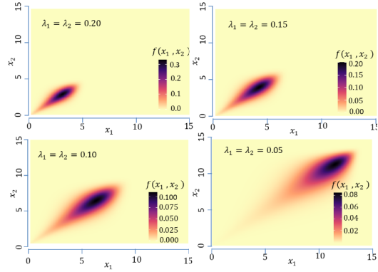
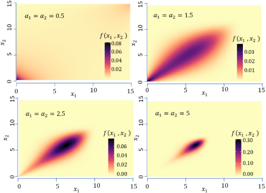
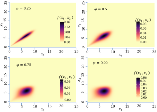
The validity of the BWED is presented in Appendix Ⅱ. Plots of the BWE density and the corresponding contour for varying parameter values are presented in
Figures 1-3.
Figure 1. Joint probability density and corresponding contour plots of the BWE density for varying values of with fixed parameters , , .
Figure 2. Joint probability density and corresponding contour plots of the BWE density for varying values of ;, with fixed parameters , , .
Figure 3. Joint probability density and corresponding contour plots of the BWE density for varying values of , with fixed parameters , , .
From
Figure 1, the plots illustrate how changes in the scale parameters influence the concentration, spread, and dependence structure of the joint distribution. In
Figure 2, the plots demonstrate the effect of the shape parameters on the skewness, tail behavior, and peak concentration of the joint density. As the shape parameters vary, the contour lines change in curvature and orientation, reflecting alterations in marginal behavior and dependence structure. In
Figure 3, the plots illustrate the role of the dependence parameter
in regulating the strength and structure of association between the two variables. As
varies, the density surface and contour configurations exhibit noticeable changes in concentration, symmetry, and dependence intensity, ranging from stronger (top-left panel) to weaker (bottom-right panel) joint interactions.
The BWE density plots together with their corresponding contour representations for the varying parameter configurations show diverse shapes observed under different parameter settings, illustrating the potential for adaptability of the BWE model in representing a wide range of bivariate data-generating processes. The contour structures further emphasize the model’s flexibility in capturing varying degrees of dependence, association patterns, and tail behavior. Collectively, these graphical features demonstrate the suitability of the BWED for modelling complex bivariate relationships encountered in practical applications, while maintaining the prescribed marginal characteristics. The generalization of the BWED to its multivariate form is given in Appendix Ⅲ.
3.2. Conditional Distributions
The conditional distribution of given can be expressed as
(4)
Conditional distributions are used in simulating the BWED via Gibb’s sampling technique in this study. They can also be used in regression and risks modelling.
3.3. Copula-based Dependence Measure
Sklar’s theorem
| [25] | A. Sklar, “Fonctions de Répartition à n Dimensions et Leurs Marges”, Publications de l'Institut de Statistique de L'Université de Paris, 1959, 8, 229-231. |
[25]
states that any multivariate joint distribution can be written in terms of univariate marginal distribution functions and a copula (link function) which describes the dependence structure between the variables. That is, for marginal cumulative distribution functions denoted by
and a joint cumulative distribution function
of random variables
, there exist a copula function,
, such that
(5)
Hence, given random variables and from the BWED with respective marginal distributions and , their copula (link) distribution and density functions are given, respectively, by
(6)
and
(7)
where , and .
One of the most desired outcomes in the study of multivariate distributions is the understanding of co-dependence structure among the variables. Unlike Pearson’s correlation, which measures straight-line relationships, monotonic dependence (often measured by the Spearman’s rho and Kendall’s tau) captures nonlinear but consistent trends. The strength of monotonic dependence is measured by copula-based Kendall’s tau, denoted by
. This can be obtained
from Eq. (
5), using
(8)
is the measure of nonlinear monotonic dependence relationship that will be used in this study. The strength of this measure as classified in www.statisticshowto.com and used in Saporu & Gongsin (2020)
| [9] | F. W. O. Saporu & I. E. Gongsin, “Modelling Dependence Relationships of Anthropometric Variables Using Copula Approach”, American Journal of Theoretical and Applied Statistics, 2020, Vol. 9, No. 5, pp. 245 - 255,
https://doi.org:10.11648/j.ajtas.20200905.18 |
[9]
is employed to aid the understanding of our interpretation.
3.4. Parameter Estimation
The EML method is used for estimation purpose. The EML method enables simultaneous estimation of all the seven parameters in the bivariate Weibull-epsilon distribution at once, using the log-likelihood function of the BWE density in Eq. (
2). This function is coded in R and executed via the optim package. The log-likelihood function for the bivariate Weibull-epsilon distribution is given by
(9)
where, is the parameter vector space and , are random samples of size .
The execution of the log-likelihood function (Eq. (
9)), simulation and other computations are carried out in R, and the script will be made available upon request.
will be computed from Eq. (
8) through numerical integration in R package, curvature.
4. Results and Discussion
4.1. Simulation
Here, we simulate data from the bivariate Weibull-epsilon distribution for given parameter values using Gibb’s sampling method. Letting
and
, we define the conditional distributions of
and that of
from Eq. (
4). Using initial value for
we simulate
from
, employ the simulated value of
into
to simulate for
. The process is repeated using the previous simulated value of one variable to simulate the next other value until the required sample size is obtained. The performance of the parameter estimates for 20 - 5,000 realizations of sampled values are presented in
Table 1.
From
Table 1, the simulation results indicate that parameter estimates improve steadily with increasing sample size, reflecting the maximum likelihood estimates’ asymptotic consistency. For small samples (
), estimates show noticeable bias and higher variability, while for larger samples (
), they converge closely to the true parameter values with markedly reduced standard errors.
Table 1. Parameter Estimates Performance of the BWED from the Sampled Bivariate Datasets.
| Parameters |
| | | | | | |
Actual values | 1.5 | 3.0 | 0.05 | 0.03 | 17.5 | 20.0 | 0.25 |
20 | 0.961 (0.173) | 3.830 (1.167) | 0.156 (0.025) | 0.048 (0.006) | 67.024 (105.64) | 15.261 (2.215) | 0.646 (0.143) |
50 | 1.452 (0.216) | 2.097 (0.355) | 0.111 (0.010) | 0.031 (0.002) | 31.274 (41.043) | 15.159 (0.226) | 0.564 (0.077) |
70 | 1.768 (0.209) | 2.456 (0.373) | 0.108 (0.007) | 0.030 (0.002) | 44.989 (88.176) | 15.193 (0.219) | 0.584 (0.067) |
100 | 2.031 (0.196) | 4.414 (0.973) | 0.100 (0.005) | 0.037 (0.004) | 27.012 (12.952) | 16.844 (1.446) | 0.628 (0.058) |
150 | 2.201 (0.205) | 3.660 (0.598) | 0.088 (0.004) | 0.032 (0.002) | 22.019 (7.077) | 16.702 (0.622) | 0.543 (0.044) |
200 | 1.938 (0.166) | 4.321 (0.556) | 0.076 (0.003) | 0.036 (0.002) | 28.545 (10.902) | 20.122 (1.307) | 0.386 (0.029) |
250 | 1.989 (0.112) | 5.004 (0.585) | 0.076 (0.002) | 0.041 (0.002) | 48.695 (23.661) | 26.819 (4.793) | 0.388 (0.025) |
500 | 1.845 (0.105) | 4.094 (0.362) | 0.068 (0.002) | 0.038 (0.002) | 28.591 (6.791) | 24.151 (2.117) | 0.304 (0.015) |
750 | 1.754 (0.063) | 3.589 (0.187) | 0.076 (0.002) | 0.039 (0.001) | 63.484 (45.204) | 23.869 (1.227) | 0.254 (0.010) |
1000 | 1.672 (0.055) | 3.481 (0.182) | 0.078 (0.002) | 0.039 (0.001) | 39.607 (10.938) | 23.408 (1.217) | 0.252 (0.009) |
1500 | 1.471 (0.042) | 2.941 (0.098) | 0.071 (0.001) | 0.036 (0.001) | 21.672 (1.308) | 20.723 (0.341) | 0.232 (0.007) |
2000 | 1.452 (0.035) | 2.968 (0.083) | 0.066 (0.001) | 0.035 (0.0004) | 19.216 (0.602) | 20.755 (0.265) | 0.236 (0.006) |
3000 | 1.420 (0.028) | 2.847 (0.066) | 0.063 (0.0008) | 0.033 (0.0003) | 18.347 (0.342) | 20.139 (0.171) | 0.233 (0.005) |
5000 | 1.501 (0.023) | 3.006 (0.054) | 0.059 (0.0006) | 0.032 (0.0003) | 18.456 (0.254) | 20.181 (0.123) | 0.248 (0.004) |
Specifically, the shape parameters () show gradual reduction in bias; improves from 0.961 (bias = − 0.359) at to 1.501 (bias = 0.0007) at , while decreases from 3.83 (bias = 0.277) to 3.006 (bias = 0.002). Standard errors shrink by nearly an order of magnitude, from nearly between 0.17 and 1.17 to nearly between 0.02 and 0.05, indicating increasing precision. Secondly, the scale parameters (,) exhibit rapid stability; converges from 0.156 (bias = 2.12) at to 0.059 (bias = 0.18) at , and from 0.048 (bias = 0.6) to 0.032 (bias = 0.067). Variability in the scale parameters decline sharply after , with standard errors falling below 0.001 for large samples. Thirdly, the location parameters () initially fluctuate widely, for example, versus the true value 17.5 at which progressively stabilize around the true values for , where at , and with biases of 0.055 and 0.009, respectively. Finally, the dependence parameter () displays consistent downward adjustment with increasing ; from 0.646 (bias = 1.58) at to 0.248 (bias = − 0.008) at , confirming convergence toward the true value 0.25. Generally, bias and variance decline monotonically across parameters, and by , all estimates closely approximate their true values. These confirm the consistency, efficiency, and robustness of the EML estimators of the BWE model under moderate to large sample sizes.
4.2. Robustness of the Bivariate Weibull-epsilon Distribution
To show the robustness of the bivariate Weibull-epsilon distribution, we compare with other bivariate distributions in the Weibull family applied in wind speed modelling, namely the bivariate Weibull distribution (BWD
1) in Villanueva et al.
| [19] | D. Villanueva, A. Feijoo & J. L.Pazos, “Multivariate Weibull Distribution for Wind Speed and Wind Power Behavior Assessment”, Resources, 2013, 2, 370 - 384,
https://doi.org:10.3390/resources2030370 |
[19]
and the bivariate Weibull distribution (BWD
2) in Monahan
. We simulated data from these distributions and fitted each to the parent distribution and the BWED. The Akaike Information Criterion (AIC) is used to determine the more compatible model.
The bivariate Weibull distributions in
| [19] | D. Villanueva, A. Feijoo & J. L.Pazos, “Multivariate Weibull Distribution for Wind Speed and Wind Power Behavior Assessment”, Resources, 2013, 2, 370 - 384,
https://doi.org:10.3390/resources2030370 |
[19]
(after modification) and
are given in Eq.s (
10) and (
11), respectively.
(10)
where and is the inverse of the error function, and
(11)
where
is the Bessel function of the order zero expressed as
| [27] | M. Abramowitz & I. A. Stegun, Handbook of Mathematical Functions, Dover, New York (1965) |
[27]
. In both Eq.s (
10) and (
11),
represents dependence, with
indicating strong to perfect correlation. Estimated results from 500 realizations of the simulated values from the two distributions are given in
Table 2.
Table 1.
Comparison of model performance for datasets simulated from two bivariate Weibull models in Eq.s (10) and (11). Density | Parameters | | |
| | | | | | | | | |
| | | | | | | | | |
| 4.866 (0.046) | 8.761 (0.131) | 4.878 (0.157) | 3.103 (0.108) | 0.206 (0.045) | | | 1907.37 | 3824.74 |
| 3.401 (0.112) | 0.142 (0.004) | 110.12 (119.80) | 2.184 (0.012) | 0.078 (0.001) | 102.44 (116.77) | 0.700 (0.029) | 1892.12 | 3798.24 |
| | | | | | | | | |
| 9.178 (0.100) | 11.005 (0.135) | 4.122 (0.033) | 3.505 (0.022) | 0.698 (0.003) | | | 2192.92 | 4395.84 |
| 4.127 (0.164) | 0.087 (0.001) | 53.138 (33.952) | 3.066 (0.279) | 0.073 (0.004) | 21.839 (7.039) | 0.993 (0.024) | 1942.04 | 3898.08 |
* actual parameter values, ** estimated parameter values (standard errors), ֎ parameters of the BWED
Table 2 compares the proposed BWED with two existing Weibull-based models developed by Villanueva et al. (
)
| [19] | D. Villanueva, A. Feijoo & J. L.Pazos, “Multivariate Weibull Distribution for Wind Speed and Wind Power Behavior Assessment”, Resources, 2013, 2, 370 - 384,
https://doi.org:10.3390/resources2030370 |
[19]
and Monahan (
)
. The comparison uses simulated datasets generated from each of these two models and evaluates performance using the AIC, where smaller AIC values indicate a better model fit. When data were generated from
, the BWED produced a lower AIC (3798.24) than the fitted
model (3824.74), showing that BWED describes the joint behavior better. The difference in AIC (
) is large enough to indicate strong support for BWED over the original model. When data were generated from BWD
2, the advantage of BWED became even more pronounced, with an AIC of 3898.08 compared to 4395.84 for
(
). The consistent superiority of BWED across both scenarios suggests that it remains reliable even when the true dependence structure differs from its own formulation. Overall, the results demonstrate that BWED is a flexible and robust model for representing joint wind-speed behavior and is therefore suited for practical environmental and renewable energy applications.
4.3. Application to Wind Speed Data
4.3.1. Motivation
Wind energy is one of the most promising alternatives to fossil fuels, offering a path to decarbonization and sustainable power generation. The growth of wind power globally has been extraordinary: for example, installed wind capacity increased from 158.5 GW in 2009 to over 542 GW by 2018
| [28] | GWEC. Global wind power boom continues despite economic woes. In: Global Wind Report 2019, pp. 8, (GWEC).
www.gwec.net |
| [29] | IRENA. Future of wind: Deployment, investment, technology, grid integration and socio-economic aspects (A Global Energy Transformation paper). International Renewable Energy Agency (2019), Abu Dhabi. www.irena.org/publications |
[28, 29]
. In 2020, wind power additions surged by approximately 93 GW, representing a 53% increase in new installations alone
| [30] | F. Zhao, “A record year for the wind industry, 2020”, In: Global Wind Report 2021, pp.6, GWEC. |
[30]
, with onshore wind capacity hitting about 699 GW
| [29] | IRENA. Future of wind: Deployment, investment, technology, grid integration and socio-economic aspects (A Global Energy Transformation paper). International Renewable Energy Agency (2019), Abu Dhabi. www.irena.org/publications |
[29]
. More recent data show that global capacity continued to grow to a total (onshore + offshore) exceeding 1000 GW by 2023
| [31] | IEA. Wind Power in 2023: Global Overview and Trends. International Energy Agency (2023), Paris. |
[31]
. This accelerating deployment is driven by urgent climate targets, falling renewable technology costs, and increased policy support.
Despite this promising growth, one of the persistent challenges in wind energy planning, forecasting, and management is the intermittent and variable nature of wind speed - both in time and across spatial locations. Wind speeds fluctuate due to meteorological variability, terrain effects, and atmospheric dynamics; and capturing their dependence structure is critical for improved prediction, site layout design, and reliability assessment of wind farms. In particular, understanding temporal dependence of wind speeds (e.g. at two different times of the same day at the same location) can reduce forecasting error and enhance wind farm modelling.
A substantial body of literature have investigated spatial dependence in wind speeds. For example, Shen et al.
| [32] | X. Shen, C. Zhou & X. Fu, “Study of Time and Meteorological Characteristics of Wind Speed Correlation in Flat Terrains Based on Operation Data”, Energies, 2018, 11, 219.
https://doi.org/10.3390/en11010219 |
[32]
examined correlations among turbines under varying meteorological conditions; Liu et al.
| [33] | S. Liu, G. Li, H. Xie & X. Wang, “Correlation Characteristic Analysis for Wind Speed in Different Geographical Hierarchies”, Energies, 2017, 10, 237.
https://doi.org/10.3390/en10020237 |
[33]
explored correlation structures, both within and between wind farms; and Kadhem et al.
| [34] | A. A. Kadhem, N. I. Abdul-Wahab, I. Aris, J. Jasni & A. N. Abdalla, “Advanced Wind Speed Prediction Model Based on a Combination of Weibull Distribution and an Artificial Neural Network”, Energies (2017), 10, 1744.
https://doi.org:10.3390/en10111744 |
[34]
associated wind variability with seasonal weather patterns. These works, however, focus predominantly on dependence across locations at the same time instant. In contrast, our interest is temporal dependence, that is modelling wind speeds at two distinct times (e.g. morning vs afternoon) recorded at the same location. This type of dependence is especially relevant in forecasting, diurnal cycle analysis, and operational decision-making.
To this end, we adopt the BWED (Eq. (
2)) to model the joint behavior of wind speeds at two time points of the same day. The key goals are: (1) fit the BWED to empirical wind speed data and quantify the degree of co-dependence between the two time-point variables; (2) compare model performance with two alternative bivariate Weibull constructions (Eqs. (
10) and (
11)); and (3) assess whether the enhanced flexibility of the BWED improves fit and/or dependence capture, in the context of wind speed data application.
4.3.2. The Data and Parameter Estimation
We analyzed daily wind speed records from Christmas Island, Australia, collected at two time points: 9:00 a.m. and 3:00 p.m of the same day. The sampling period spans from October 1, 2018 to March 25, 2020. Days with missing observations at either time point were removed, yielding 517 complete bivariate observations out of an initial 542 days. The original measurements reported in km/h were transformed to m/s using a conversion factor of 0.278. The data source is 错误!超链接引用无效。
The descriptive statistics of the wind speed data are given in
Table 3.
Table 3. Descriptive Statistics of the Wind Speed.
Time | Min | | | | | Max |
9 a. m. | 0.56 | 3.61 | 5.28 | 5.01 | 6.12 | 9.17 |
3 p. m. | 1.11 | 3.61 | 4.73 | 4.84 | 6.12 | 8.34 |
cor = 0.807
The descriptive summaries in
Table 3 indicates positive correlation between the wind speeds at 9 a. m. and 3 p. m.
We fitted three models to the data, namely: the proposed BWED model (Eq. (
2)); the bivariate Weibull model in Villanueva et al.
| [19] | D. Villanueva, A. Feijoo & J. L.Pazos, “Multivariate Weibull Distribution for Wind Speed and Wind Power Behavior Assessment”, Resources, 2013, 2, 370 - 384,
https://doi.org:10.3390/resources2030370 |
[19]
(Eq. (
10)); and the bivariate Weibull model in Monahan
(Eq. (
11)). For all the models, parameters were estimated using maximum likelihood method. In the BWED and Villanueva
| [19] | D. Villanueva, A. Feijoo & J. L.Pazos, “Multivariate Weibull Distribution for Wind Speed and Wind Power Behavior Assessment”, Resources, 2013, 2, 370 - 384,
https://doi.org:10.3390/resources2030370 |
[19]
model cases, we maximized the log-likelihood (Eq. 9) using the optim package in R. For Monahan’s model
, estimation encountered identifiability or likelihood surface irregularities, thus, the three parameters (
) were estimated via direct maximization, while the remaining two parameters (
) were located by examining the profile of the log-likelihood surfaces, holding other parameters fixed. The models’ fit and parameter estimates are summarized in
Tables 4 and 5.
Table 4. Maximum likelihood estimates and Wald significance tests for the parameters of the BWED fitted to Christmas Island wind speed data.
Parameter | | | | | | | |
Estimate | 1.890 | 0.107 | 10.988 | 2.199 | 0.118 | 12.874 | 0.417 |
Std error | 0.096 | 0.003 | 0.655 | 0.128 | 0.004 | 1.872 | 0.019 |
Wald stat | 19.618 | 36.267 | 16.780 | 17.201 | 32.065 | 6.877 | 22.064 |
p-value | 0.000 | 0.000 | 0.000 | 0.000 | 0.000 | 0.000 | 0.000 |
Remark | Sig | Sig | Sig | Sig | Sig | Sig | Sig |
Sig = significant, ,
Table 5. Comparative fit results for competing bivariate Weibull-type models fitted to the Christmas Island wind speed data.
Density | Parameters | | |
| | | | | | | |
| 5.930 (0.081) | 5.726 (0.082) | 3.243 (0.114) | 3.431 (0.132) | 0.927 (0.003) | 2123.99 | 4257.98 |
| | | | | | | |
| 5.606 (0.076) | 5.387 (0.067) | 3.197 (0.112) | 3.477 (0.120) | 0.390 (0.036) | 1938.36 | 3886.72 |
All estimated parameter values are statistically significant. The marginal shape parameters (, ) are highly significant and confirm that the wind-speed distributions are not memoryless and exhibit pronounced peaks, a characteristic commonly observed in Weibull-type wind speed behavior. The scale parameters (, ) are also statistically significant, indicating their importance in shaping the tail behavior and variability of wind speeds. The location parameters (, ) reflect the physical limits of observed wind speeds and provide realistic bounds for extreme values. The estimated dependence parameter () is precise and significant, indicating moderate nonlinear dependence between the paired wind speed measurements of the same day. This suggests that wind speeds observed at different times of the day exhibit some noticeable degree of persistence, while still retaining variability.
Compared to the dependence measure formulations proposed by Villanueva et al.
| [19] | D. Villanueva, A. Feijoo & J. L.Pazos, “Multivariate Weibull Distribution for Wind Speed and Wind Power Behavior Assessment”, Resources, 2013, 2, 370 - 384,
https://doi.org:10.3390/resources2030370 |
[19]
and Monahan
, with estimates presented in
Table 5, the BWED’s presentation captures the nonlinear dependence characteristics of the two times of the day much better. Their dependence parameters (
and
, respectively) imply strong and relatively weak linear dependence.
Model comparison using the AIC clearly favours the BWED (AIC = 3468.56) over (4257.98) and (3886.72). The large AIC differences ( and , respectively) provide strong evidence that the BWED offers a substantially better representation of the joint wind-speed behavior. This improved fit likely arises from its flexible survival-based dependence structure and the ability to capture nonlinear association.
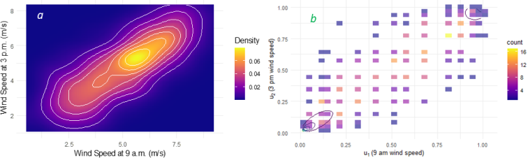
Given its superior fit and realistic dependence characterization, the BWED is adopted for subsequent dependence visualization, including the copula-based plots shown in
Figure 4 and drawing of inference from application of model to data.
Figure 4. Copula-based visualization of wind speed dependence at Christmas Island, Australia. Panel.
From
Figure 4, panel
(a) presents the copula-based joint density contours for wind speeds measured at 9 a.m. (x-axis) and 3 p.m. (y-axis) at Christmas Island. The contour orientation along the 45° diagonal axis signifies some degree of positive dependence between the two time periods. This indicates that higher morning wind speeds are likely associated with higher afternoon wind speeds, reflecting to some extent temporal persistence of wind regimes over the location. The dense yellow-to-orange region (4 - 6 m/s) marks the area of highest joint probability, implying that moderate wind speeds dominate the daily wind profile. The smooth gradient and absence of outlying contour distortion suggest that the BWE copula adequately captures the underlying dependence structure without overestimating tail co-movement. Panel
(b) shows the empirical copula representation of the same dataset, with axes
and
denoting the pseudo-observations transformed to the unit square
. The color intensity represents the frequency of paired observations, and the overlaid contour lines correspond to the BWE copula density in the copula domain. The clustering of points along the main diagonal confirms monotonic co-movement, and the contour overlay demonstrates a close alignment between the empirical dependence pattern and the theoretical BWE copula density; an indicator of good model calibration. The few sparse points near the corners (high-high and low-low regions) suggest mild tail dependence.
Finally, the good overlap (Panel
a) between the empirical and theoretical contours provides a supporting visual evidence of the goodness-of-fit of the BWED. Also,
Figure 4b is indicative of a consistent graphical evidence that the BWED offers an adequate representation of the co-dependence structure in the Australian wind speed data.
4.3.3. Dependence Measure
The copula-based measure of monotonic dependence used here is Kendall’s tau
. Monotonic dependence refers to how two variables consistently move in the same relative direction (positive) or opposite direction (negative), but not necessarily at a constant rate. Unlike linear relationships, monotonic trends can curve, so long as they never reverse direction. This estimate is presented in
Table 6 together with the classification of the strength of this measure as used in
| [9] | F. W. O. Saporu & I. E. Gongsin, “Modelling Dependence Relationships of Anthropometric Variables Using Copula Approach”, American Journal of Theoretical and Applied Statistics, 2020, Vol. 9, No. 5, pp. 245 - 255,
https://doi.org:10.11648/j.ajtas.20200905.18 |
[9]
.
Table 6. Estimate of co-dependence measure of BWED for Wind speed data.
Method | | Strength |
EML | 0.583 | Moderate |
From
Table 6, the value obtained indicates that there is a moderate positive monotonic dependence between the wind speeds at the two time points of the day. This implies that the tendency of one variable to increase with the other is visible but there is a significant variation in the data which is clearly evident in
Figure 4b.
4.4. Discussion of Results
The new bivariate non-normal probability density function generated in this study, referred to as the BWED, describes the simultaneous occurrences of two random phenomena, each assumed to be characterized by the univariate Weibull-epsilon distribution
| [41] | I. E. Gongsin & F. W. O. Saporu, “The Weibull-epsilon distribution - its properties and applications”, International Journal of Mathematical and Computational Methods, volume 5, 2020, pp 80 - 88. http://www.iaras.org/iaras/journals/ijmcm |
[41]
. The shapes of the bivariate density function, shown in
Figures 1-3, at varying parameter values, depict different random simultaneous occurrences in nature, thus providing visual evidence of its flexibility to describe the intermittence in natural processes.
The simulation results confirm that the EML estimators yields consistent and efficient estimates for the parameters of the new bivariate distribution. Across sample sizes from 20 to 5,000, the estimates approach the true values monotonically, with both bias and standard error diminishing as
increases. This convergence behavior validates the asymptotic properties of the EML estimators and demonstrates its reliability even under moderate sample conditions typical of environmental data. The accurate recovery of the dependence parameter
, which converged from 0.646 at
to approximately 0.25 at
, underscores the method’s effectiveness in capturing dependence structures crucial for joint risk and reliability modelling. Similar improvements in convergence and variance reduction have been reported in recent MCMC-based estimation frameworks for copula and compound distributions applied to wind and hydrological data
| [35] | S. Huang, Q. S. Li, Z. Shu & P. W. Chan, “Copula-based estimation of directional extreme wind speeds: Application for wind-resistant structural design”, Structures 60(4):105845, 2024. https://doi.org/10.1016/j.istruc.2023.105845 |
| [36] | H. Qasem, N-E. Joergensen, A. Rahman, H. A. Samman, S. Al-Malki & A. S. Al-Ansari, “Vine Copula-Based Multivariate Distribution of Rainfall Intensity, Wind Speed, and Wind Direction for Optimizing Qatari Meteorological Stations”, Water, 16(9):1257, 2024, https://doi.org/10.3390/w16091257 |
[35, 36]
.
Comparative analysis with existing bivariate Weibull models further emphasizes the robustness of the BWED. The log-likelihood and AIC results show that the proposed BWED is consistently more amenable to data compared to the bivariate Weibull models in Villanueva et al.
| [19] | D. Villanueva, A. Feijoo & J. L.Pazos, “Multivariate Weibull Distribution for Wind Speed and Wind Power Behavior Assessment”, Resources, 2013, 2, 370 - 384,
https://doi.org:10.3390/resources2030370 |
[19]
and Monahan
, confirming a better flexibility in modelling both central and mild tail dependence. This advantage arises from the epsilon component, which adjusts the joint tail thickness without distorting marginal behavior, thereby offering a more adaptable dependence structure. Such flexibility has also been highlighted in recent studies where hybrid or copula-based Weibull models yielded improved fits in meteorological and renewable energy datasets
| [37] | W. Wang, F. Chen, Y. Li & L. Weng, “A hybrid WOA-KDE and mixed copula framework for directional wind assessment in complex terrain”, Sustainable Energy Technologies and Assessments, 83, 2025, 104590.
https://doi.org/10.1016/j.seta.2025.104590 |
| [38] | S. Huang, Q. Li, Z. Shu, & P. W. Chan, “Copula-based joint distribution analysis of wind speed and wind direction: Wind energy development for Hong Kong”, Wind Energy, 26(9), 2023, 900 - 922. https://doi.org/10.1002/we.2847 |
[37, 38]
. These findings suggest that the BWED can serve as a general framework for multivariate modelling where marginal Weibull behavior is evident but dependence deviates from conventional Gaussian or Gumbel copula assumptions.
The empirical application to wind speed data from Christmas Island further demonstrates the practical usefulness of the proposed BWED model. Graphical validation through contour density and empirical copula plots shows strong agreement between the theoretical BWED copula and the empirical pseudo-observations, indicating a well-calibrated model with little evidence of misfit. Similar copula-based diagnostics have shown that such approaches effectively capture nonlinear dependence structures in energy-related variables
| [39] | T. E. B. de Carvalho Silva, P. Maçaira, F. L. Cyrino Oliveira, & G. A. A. Pereira, “Enhancing energy planning with copula-based dependency models”, Energy Reports, Vol. 14, (2025), Pages 43-55. https://doi.org/10.1016/j.egyr.2025.05.028 |
[39]
. The marginal shape parameter estimates (
) indicate typical Weibull-type behavior with clear nonzero modes, consistent with observed wind speed distributions.
The dependence parameter () is significant and reflects moderate nonlinear co-movement driven by shared atmospheric conditions. The estimate of the copula-based Kendall’s tau, , suggests that this co-movement is a moderate positive monotonic dependence. Consequently, other meteorological and atmospheric factors (humidity, temperature, etc.) are influencing morning wind speed alongside that of the afternoon of the same day causing more noise in the data than a strong relationship.
There are practical insights provided by the nature of this dependence. These are:
1) Morning wind speed contain to some extent predictive information for corresponding afternoon conditions. This can improve the skill of short-term wind power forecasts and enable more reliable scheduling of maintenance or storage operations.
2) Wind power variability in the morning is likely to be mirrored later in the day, a feature critical for grid stability assessment.
3) The dependence relationship captured by the BWED copula allows realistic simulation of the joint wind profiles, aiding probabilistic forecasting and uncertainty quantification in renewable energy integration.
These insights align with recent developments emphasizing dependence-focused stochastic modelling in power systems and atmospheric sciences
| [35] | S. Huang, Q. S. Li, Z. Shu & P. W. Chan, “Copula-based estimation of directional extreme wind speeds: Application for wind-resistant structural design”, Structures 60(4):105845, 2024. https://doi.org/10.1016/j.istruc.2023.105845 |
| [36] | H. Qasem, N-E. Joergensen, A. Rahman, H. A. Samman, S. Al-Malki & A. S. Al-Ansari, “Vine Copula-Based Multivariate Distribution of Rainfall Intensity, Wind Speed, and Wind Direction for Optimizing Qatari Meteorological Stations”, Water, 16(9):1257, 2024, https://doi.org/10.3390/w16091257 |
[35, 36]
.
From a methodological standpoint, the results confirm that the BWED combines parsimony with flexibility, providing a tractable yet expressive model for wind-speed dependence. Its superior AIC performance over traditional bivariate Weibull formulations suggests that accounting for mild tail dependence significantly improves model fit. Furthermore, the copula representation inherent in the BWED framework allows its direct extension to higher dimensions, making it suitable for spatiotemporal modelling of wind data across multiple sites or time intervals. Given the increasing complexity of renewable energy systems, such scalable dependence models are becoming essential for integrated forecasting and risk management.
These findings are also timely given the rapid global expansion of wind power. According to recent reports by the Global Wind Energy Council
| [40] | GWEC. Global Wind Report 2024. Global Wind Energy Council (2024), Brussels. |
[40]
and the International Energy Agency
| [31] | IEA. Wind Power in 2023: Global Overview and Trends. International Energy Agency (2023), Paris. |
[31]
, global installed wind capacity surpassed 1,000 GW by 2023, with continued double-digit annual growth. This accelerating deployment heightens the need for accurate probabilistic models of wind dependence to support grid balancing, energy market forecasting, and investment risk analysis. As renewable penetration increases, the cost of misestimating joint variability also rises, making advanced dependence models like the BWE particularly valuable for operational planning and reliability studies.
Notwithstanding its strengths, several limitations suggest directions for further research. The present analysis assumes temporal stationarity and constant dependence; extending the BWED to time-varying or regime-switching frameworks could better capture evolving dependence structures. Although AIC-based selection establishes relative fit, out-of-sample validation using cross-validated forecast accuracy would provide stronger evidence of predictive performance. Future studies may incorporate meteorological covariates - such as atmospheric pressure, humidity, or stability indices - into the marginal or copula components and evaluate the BWED alongside alternative copula families to assess robustness. For extreme-event analysis, tail-adaptive or vine copula extensions could improve characterization of joint wind extremes across spatially correlated sites. Further work could also explore spatio-temporal formulations and applications in hydrology and reliability engineering, where modeling dependent extremes and component lifetimes is essential.
Appendix: The Bivariate Weibull-epsilon Distribution and Its Multivariate Form
Appendix Ⅰ: Derivation of the Bivariate Weibull-epsilon Distribution
The Weibull-epsilon distribution was introduced
| [41] | I. E. Gongsin & F. W. O. Saporu, “The Weibull-epsilon distribution - its properties and applications”, International Journal of Mathematical and Computational Methods, volume 5, 2020, pp 80 - 88. http://www.iaras.org/iaras/journals/ijmcm |
[41]
as a life time distribution with flexible shapes within its parameter range that can be used as density and hazard rate functions. For a random variable
, its density and distribution functions are, respectively, given by
(A-1)
and
(A-2)
where , , .
The bivariate Weibull-epsilon distribution is constructed using the joint survival function method defined in Eq. (
1). The Weibull-epsilon cumulative failure rate function,
, is obtained as
(A-3)
For simplification of notation, let . Then the Weibull-epsilon joint survival rate function is given by
(A-4)
Differentiating
with respect to
and
gives the bivariate Weibull-epsilon probability density function in Eq. (
2). The corresponding cumulative distribution function is derived as
The bivariate Weibull-epsilon distribution function can be determined from the relationship between bivariate cumulative distribution and survival functions. This is given
by
,
(A-5)
Substituting
and
into
, the bivariate Weibull-epsilon distribution function is obtained, and given in Eq.(
3).
Appendix Ⅱ: Validity of the BWED
Theorem
The bivariate Weibull-epsilon density function,
, given in Eq. (
2) is a true probability density function.
Proof
It suffices to show that .
Since and , then
Also
Since is a strictly monotonic increasing function, the proof is complete.
Appendix Ⅲ: Multivariate Weibull-epsilon distribution
The bivariate Weibull-epsilon distribution can be generalized to its multivariate form by the expansion of the expression of the bivariate survival function
. That is, given an
dimemsional random vector
, the joint survival function is given by
(A-6)
And for a Weibull-epsilon random vector, , the joint survival function is given by
(A-7)
where , , and .
The multivariate Weibull-epsilon probability density function is derived from the joint survival function (
) by differentiation
. That is,
(A-8)
where number of summands of the partition of such that , , ,
is the falling factorial of ,
total number of partitions of , and
total number of set partitions of the set corresponding to the partition of .





 Share This Article
 Twitter
 Linked In
 Facebook
 Copy
Copy Download