The uneven distribution of primary sources of electric power generation in Economic Community of West African States (ECOWAS) compelled the heads of states to create the West African Power Pool (WAPP). The vision of this system is to set up a common electrical energy market to satisfy the balance between supply and demand at an affordable price using the interconnected network. Forecasting maximum power demand and energy consumption is essential for planning and the coordination of new power plant and transmission lines building. This work consists of predicting maximum power demand and total energy that must transit through the WAPP interconnected network by the year 2032. We compare the performances of three time series models namely the Long Short-Term Memory (LSTM), Auto-Regressive Integrated Moving Average (ARIMA) and Fb Facebook Prophet. Electric power and energy data used for training the systems comes from the WAPP authorties. The results show that, for monthly peaks, the Facebook (Fb) Prophet model is the best, with a MAPE (mean absolute error percentage) of 3.1% and a low RMSE (root mean square error) of 1.225 GW. For energy prediction, ARIMA performances are the best compared to others with (RMSE 1.20 TWh, MAPE 1.00%). Thus, the forecast for total annual energy consumption and annual peak demand will be, respectively, 96.85TWh and 13.6 GW in 2032.
| Published in | International Journal of Energy and Power Engineering (Volume 13, Issue 2) |
| DOI | 10.11648/j.ijepe.20241302.11 |
| Page(s) | 21-31 |
| Creative Commons |
This is an Open Access article, distributed under the terms of the Creative Commons Attribution 4.0 International License (http://creativecommons.org/licenses/by/4.0/), which permits unrestricted use, distribution and reproduction in any medium or format, provided the original work is properly cited. |
| Copyright |
Copyright © The Author(s), 2024. Published by Science Publishing Group |
Power Demand, Energy Supply, Maximum Power Peak, Forecasting, Energy Planning, Interconnected Network
2.1. Forecasting Method with ARIMA
2.2. Forecasting Method with Prophet
2.3. LSTM Forecasting Method
PERFORMANCE | MAPE (%) | RMSE (GW) |
|---|---|---|
ARIMA | 4,59 | 1,276 |
PROPHET | 3,10 | 1,255 |
LSTM | 3,17 | 1,259 |
Month | 1 | 2 | 3 | 4 | 5 | 6 | 7 | 8 | 9 | 10 | 11 | 12 |
|---|---|---|---|---|---|---|---|---|---|---|---|---|
GW | 13,45 | 13,49 | 13,37 | 13,25 | 13,18 | 13,13 | 13,17 | 13,18 | 13,19 | 13,3 | 13,52 | 13,6 |
PERFORMANCE | MAPE (%) | RMSE (TWh) |
|---|---|---|
ARIMA | 1,00 | 1,20 |
PROPHET | 4,19 | 3,24 |
| [1] | L. K. Lim, Z. A. Muis, W. S. Ho, H. Hashim, and C. P. C. Bong, “Review of the energy forecasting and scheduling model for electric buses,” Energy, vol. 263, p. 125773, 2023, |
| [2] | M. Q. Raza and A. Khosravi, “A review on artificial intelligence based load demand forecasting techniques for smart grid and buildings,” Renewable and Sustainable Energy Reviews, vol. 50. Elsevier Ltd, pp. 1352–1372, Jun. 18, 2015. |
| [3] | J. Pérez-García and J. Moral-Carcedo, “Analysis and long term forecasting of electricity demand trough a decomposition model: A case study for Spain,” Energy, vol. 97, pp. 127–143, Feb. 2016, |
| [4] | S. Ghosh and A. Das, “Short-run electricity demand forecasts in Maharashtra,” Appl. Econ., vol. 34, no. 8, pp. 1055–1059, 2002, |
| [5] | S. R. Rallapalli and S. Ghosh, “Forecasting monthly peak demand of electricity in India-A critique,” Energy Policy, vol. 45, pp. 516–520, Jun. 2012, |
| [6] | H. K. Alfares and M. Nazeeruddin, “Electric load forecasting: Literature survey and classification of methods,” Int. J. Syst. Sci., vol. 33, no. 1, pp. 23–34, Jan. 2002, |
| [7] | Aucoin and Frédérik, “Analyse de la demande d’électricité du secteur résidentiel du Québec,” 2007. |
| [8] | J. P. Lévy, N. Roudil, A. Flamand, and F. Belaïd, “The determinants of domestic energy consumption,” Flux, vol. 96, no. 2, pp. 40–54, 2014, |
| [9] | A. M. Masih and R. Masih, “Energy consumption, real income and temporal causality: results from a multi-country study based on cointegration and error-correction modelling techniques,” 1996. |
| [10] | R. Mahadevan and J. Asafu-Adjaye, “Energy consumption, economic growth and prices: A reassessment using panel VECM for developed and developing countries,” Energy Policy, vol. 35, no. 4, pp. 2481–2490, Apr. 2007, |
| [11] | S. Yu, K. Zhu, and X. Zhang, “Energy demand projection of China using a path-coefficient analysis and PSO-GA approach,” Energy Convers. Manag., vol. 53, no. 1, pp. 142–153, Jan. 2012, |
| [12] | N. A. Mohammed, “Modelling of unsuppressed electrical demand forecasting in Iraq for long term,” Energy, vol. 162, pp. 354–363, Nov. 2018, |
| [13] | D. Angelopoulos, Y. Siskos, and J. Psarras, “Disaggregating time series on multiple criteria for robust forecasting: The case of long-term electricity demand in Greece,” Eur. J. Oper. Res., vol. 275, no. 1, pp. 252–265, May 2019, |
| [14] | A. Veit, C. Goebel, R. Tidke, C. Doblander, and H. A. Jacobsen, “Household electricity demand forecasting - Benchmarking state-of-the-art methods,” e-Energy 2014 - Proc. 5th ACM Int. Conf. Futur. Energy Syst., pp. 233–234, 2014, |
| [15] | “NASA POWER | Prediction Of Worldwide Energy Resources.” [Online]. Available: |
| [16] | “World Bank Open Data | Data.” [Online]. Available: |
| [17] | C. Kuster, Y. Rezgui, and M. Mourshed, “Electrical load forecasting models: A critical systematic review,” Sustainable Cities and Society, vol. 35. Elsevier Ltd, pp. 257–270, Nov. 01, 2017. |
| [18] | N. Wei, C. Li, X. Peng, F. Zeng, and X. Lu, “Conventional models and artificial intelligence-based models for energy consumption forecasting: A review,” J. Pet. Sci. Eng., vol. 181, Oct. 2019, |
| [19] | T. Ahmad, H. Zhang, and B. Yan, “A review on renewable energy and electricity requirement forecasting models for smart grid and buildings,” Sustainable Cities and Society, vol. 55. Elsevier Ltd, Apr. 01, 2020. |
| [20] | M. A. Hammad, B. Jereb, B. Rosi, and D. Dragan, “Methods and Models for Electric Load Forecasting: A Comprehensive Review,” Logist. Sustain. Transp., vol. 11, no. 1, pp. 51–76, 2020, |
| [21] | S. Asumadu-Sarkodie and P. A. Owusu, “Forecasting Nigeria’s energy use by 2030, an econometric approach,” Energy Sources, Part B Econ. Plan. Policy, vol. 11, no. 10, pp. 990–997, 2016, |
| [22] | E. Caro, J. Juan, and J. Cara, “Periodically correlated models for short-term electricity load forecasting,” Appl. Math. Comput., vol. 364, Jan. 2020, |
| [23] | S. A. Sarkodie, “Estimating Ghana’s electricity consumption by 2030: An ARIMA forecast,” Energy Sources, Part B Econ. Plan. Policy, vol. 12, no. 10, pp. 936–944, Oct. 2017, |
| [24] | S. Ozturk and F. Ozturk, “Prediction of Energy Consumption of Turkey on Sectoral Bases by Arima Model,” Energy Econ. Lett., vol. 5, no. 1, pp. 23–30, 2018, |
| [25] | L. E. Architecture, Z. Wang, X. Su, and Z. Ding, “Long-Term Traffic Prediction Based on,” Ieee Trans. Intell. Transp. Syst., vol. 22, no. 10, pp. 1–11, 2020. |
| [26] | E. Chodakowska, J. Nazarko, Ł. Nazarko, H. S. Rabayah, R. M. Abendeh, and R. Alawneh, “ARIMA Models in Solar Radiation Forecasting in Different Geographic Locations,” Energies, vol. 16, no. 13, 2023, |
| [27] | I. G. I. Sudipa, R. Riana, I. N. T. A. Putra, C. P. Yanti, and M. D. W. Aristana, “Trend Forecasting of the Top 3 Indonesian Bank Stocks Using the ARIMA Method,” SinkrOn, vol. 8, no. 3, pp. 1883–1893, 2023, |
| [28] | S. Shahin, M. Roshdy, and M. Omar, “Predicting the Monthly Average Price (LE/KG) For Egyptian Broiler Farms (2019–2022) Using Auto regressive Integrated-Moving-Average (ARIMA) Model,” Zagazig Vet. J., vol. 51, no. 1, pp. 27–44, 2023, |
| [29] | J. Sharma et al., “A novel long term solar photovoltaic power forecasting approach using LSTM with Nadam optimizer: A case study of India,” Energy Sci. Eng., vol. 10, no. 8, pp. 2909–2929, 2022, |
| [30] | W. Kong, Z. Y. Dong, Y. Jia, D. J. Hill, Y. Xu, and Y. Zhang, “Short-Term Residential Load Forecasting Based on LSTM Recurrent Neural Network,” IEEE Trans. Smart Grid, vol. 10, no. 1, pp. 841–851, 2019, |
| [31] | W. Kong, Z. Y. Dong, D. J. Hill, F. Luo, and Y. Xu, “Short-term residential load forecasting based on resident behaviour learning,” IEEE Trans. Power Syst., vol. 33, no. 1, pp. 2016–2017, 2018, |
| [32] | I. Kumar, B. K. Tripathi, and A. Singh, “Attention-based LSTM network-assisted time series forecasting models for petroleum production,” Eng. Appl. Artif. Intell., vol. 123, p. 106440, 2023, |
| [33] | D. K. Dhaked, S. Dadhich, and D. Birla, “Power output forecasting of solar photovoltaic plant using LSTM,” Green Energy Intell. Transp., vol. 2, no. 5, p. 100113, 2023, |
| [34] | A. Docheshmeh Gorgij, G. Askari, A. A. Taghipour, M. Jami, and M. Mirfardi, “Spatiotemporal Forecasting of the Groundwater Quality for Irrigation Purposes, Using Deep Learning Method: Long Short-Term Memory (LSTM),” Agric. Water Manag., vol. 277, p. 108088, 2023, |
| [35] | C. Long, C. Yu, and T. Li, “Prophet-Based Medium and Long-Term Electricity Load Forecasting Research,” J. Phys. Conf. Ser., vol. 2356, no. 1, pp. 0–8, 2022, |
| [36] | A. I. Almazrouee, A. M. Almeshal, A. S. Almutairi, M. R. Alenezi, and S. N. Alhajeri, “Long-term forecasting of electrical loads in Kuwait using prophet and holt-winters models,” Appl. Sci., vol. 10, no. 16, Aug. 2020, |
| [37] | M. K. Islam, N. M. S. Hassan, M. G. Rasul, K. Emami, and A. A. Chowdhury, “Forecasting of Solar and Wind Resources for Power Generation,” Energies, vol. 16, no. 17, 2023, |
| [38] | B. Türkmen, S. Kır, and N. C. Türkmen, “Forecasting Electricity Prices for the Feasibility of Renewable Energy Plants BT - Advances in Intelligent Manufacturing and Service System Informatics,” Z. Şen, Ö. Uygun, and C. Erden, Eds., Singapore: Springer Nature Singapore, 2024, pp. 783–793. |
| [39] | B. J. Mughal et al., “Modeling and simulation for the second wave of COVID-19 in Pakistan,” Res. Biomed. Eng., 2024, |
| [40] |
“WAPP Annual Report 2020 | ECOWAPP.”
https://www.ecowapp.org/en/documents/wapp-annual-report-2020 (accessed Feb. 14, 2024). |
| [41] |
“Rapport annuel 2021 | ECOWAPP.”
https://www.ecowapp.org/en/node/922 (accessed Feb. 14, 2024). |
| [42] |
“WAPP Annual Report 2019 | ECOWAPP.”
https://www.ecowapp.org/en/documents/wapp-annual-report-2019 (accessed Feb. 14, 2024). |
| [43] | D. Rosadi, “New Procedure for Determining Order of Subset Autoregressive Integrated Moving Average (ARIMA) Based on Over-fitting Concept.” [Online]. Available: www.bps.go.id |
| [44] | M. A. Villegas and D. J. Pedregal, “Automatic selection of unobserved components models for supply chain forecasting,” Int. J. Forecast., vol. 35, no. 1, pp. 157–169, Jan. 2019, |
| [45] | O. O. Awe, A. Okeyinka, and J. O. Fatokun, “An Alternative Algorithm for ARIMA Model Selection,” in 2020 International Conference in Mathematics, Computer Engineering and Computer Science, ICMCECS 2020, Institute of Electrical and Electronics Engineers Inc., Mar. 2020. |
| [46] | T. M. Awan and F. Aslam, “Prediction of daily COVID-19 cases in European countries using automatic ARIMA model,” 2020. [Online]. Available: |
| [47] | X. H. Le, H. V. Ho, G. Lee, and S. Jung, “Application of Long Short-Term Memory (LSTM) neural network for flood forecasting,” Water (Switzerland), vol. 11, no. 7, 2019, |
| [48] | A. Włodarczyk, “X-13-ARIMA-SEATS jako narzędzie wspomagające proces zarządzania środowiskowego w elektrowni,” Polish J. Manag. Stud., vol. 16, no. 1, pp. 280–291, 2017, |
| [49] | B. Lénárt, “Automatic identification of ARIMA models with neural network,” Period. Polytech. Transp. Eng., vol. 39, no. 1, pp. 39–42, 2011, |
| [50] | I. K. Nti, M. Teimeh, O. Nyarko-Boateng, and A. F. Adekoya, “Electricity load forecasting: a systematic review,” J. Electr. Syst. Inf. Technol., vol. 7, no. 1, 2020, |
APA Style
Prodjinotho, U. T., Chetangny, P. K., Agbomahena, M. B., Zogbochi, V., Medewou, L., et al. (2024). Long Term Forecasting of Peak Demand and Annual Electricity Consumption of the West African Power Pool Interconnected Network by 2032. International Journal of Energy and Power Engineering, 13(2), 21-31. https://doi.org/10.11648/j.ijepe.20241302.11
ACS Style
Prodjinotho, U. T.; Chetangny, P. K.; Agbomahena, M. B.; Zogbochi, V.; Medewou, L., et al. Long Term Forecasting of Peak Demand and Annual Electricity Consumption of the West African Power Pool Interconnected Network by 2032. Int. J. Energy Power Eng. 2024, 13(2), 21-31. doi: 10.11648/j.ijepe.20241302.11
AMA Style
Prodjinotho UT, Chetangny PK, Agbomahena MB, Zogbochi V, Medewou L, et al. Long Term Forecasting of Peak Demand and Annual Electricity Consumption of the West African Power Pool Interconnected Network by 2032. Int J Energy Power Eng. 2024;13(2):21-31. doi: 10.11648/j.ijepe.20241302.11
@article{10.11648/j.ijepe.20241302.11,
  author = {Ulrich Thierry Prodjinotho and Patrice Koffi Chetangny and Macaire Bienvenu Agbomahena and Victor Zogbochi and Laurent Medewou and Gerald Barbier and Didier Chamagne},
  title = {Long Term Forecasting of Peak Demand and Annual Electricity Consumption of the West African Power Pool Interconnected Network by 2032
},
  journal = {International Journal of Energy and Power Engineering},
  volume = {13},
  number = {2},
  pages = {21-31},
  doi = {10.11648/j.ijepe.20241302.11},
  url = {https://doi.org/10.11648/j.ijepe.20241302.11},
  eprint = {https://article.sciencepublishinggroup.com/pdf/10.11648.j.ijepe.20241302.11},
  abstract = {The uneven distribution of primary sources of electric power generation in Economic Community of West African States (ECOWAS) compelled the heads of states to create the West African Power Pool (WAPP). The vision of this system is to set up a common electrical energy market to satisfy the balance between supply and demand at an affordable price using the interconnected network. Forecasting maximum power demand and energy consumption is essential for planning and the coordination of new power plant and transmission lines building. This work consists of predicting maximum power demand and total energy that must transit through the WAPP interconnected network by the year 2032. We compare the performances of three time series models namely the Long Short-Term Memory (LSTM), Auto-Regressive Integrated Moving Average (ARIMA) and Fb Facebook Prophet. Electric power and energy data used for training the systems comes from the WAPP authorties. The results show that, for monthly peaks, the Facebook (Fb) Prophet model is the best, with a MAPE (mean absolute error percentage) of 3.1% and a low RMSE (root mean square error) of 1.225 GW. For energy prediction, ARIMA performances are the best compared to others with (RMSE 1.20 TWh, MAPE 1.00%). Thus, the forecast for total annual energy consumption and annual peak demand will be, respectively, 96.85TWh and 13.6 GW in 2032.
},
 year = {2024}
}
TY  - JOUR
T1  - Long Term Forecasting of Peak Demand and Annual Electricity Consumption of the West African Power Pool Interconnected Network by 2032

AU  - Ulrich Thierry Prodjinotho
AU  - Patrice Koffi Chetangny
AU  - Macaire Bienvenu Agbomahena
AU  - Victor Zogbochi
AU  - Laurent Medewou
AU  - Gerald Barbier
AU  - Didier Chamagne
Y1  - 2024/04/02
PY  - 2024
N1  - https://doi.org/10.11648/j.ijepe.20241302.11
DO  - 10.11648/j.ijepe.20241302.11
T2  - International Journal of Energy and Power Engineering
JF  - International Journal of Energy and Power Engineering
JO  - International Journal of Energy and Power Engineering
SP  - 21
EP  - 31
PB  - Science Publishing Group
SN  - 2326-960X
UR  - https://doi.org/10.11648/j.ijepe.20241302.11
AB  - The uneven distribution of primary sources of electric power generation in Economic Community of West African States (ECOWAS) compelled the heads of states to create the West African Power Pool (WAPP). The vision of this system is to set up a common electrical energy market to satisfy the balance between supply and demand at an affordable price using the interconnected network. Forecasting maximum power demand and energy consumption is essential for planning and the coordination of new power plant and transmission lines building. This work consists of predicting maximum power demand and total energy that must transit through the WAPP interconnected network by the year 2032. We compare the performances of three time series models namely the Long Short-Term Memory (LSTM), Auto-Regressive Integrated Moving Average (ARIMA) and Fb Facebook Prophet. Electric power and energy data used for training the systems comes from the WAPP authorties. The results show that, for monthly peaks, the Facebook (Fb) Prophet model is the best, with a MAPE (mean absolute error percentage) of 3.1% and a low RMSE (root mean square error) of 1.225 GW. For energy prediction, ARIMA performances are the best compared to others with (RMSE 1.20 TWh, MAPE 1.00%). Thus, the forecast for total annual energy consumption and annual peak demand will be, respectively, 96.85TWh and 13.6 GW in 2032.

VL  - 13
IS  - 2
ER  -
Laboratory of Electrotechnics, Telecommunications and Applied Computing, University of Abomey-Calavi, Abomey-Calavi, Benin
Laboratory of Electrotechnics, Telecommunications and Applied Computing, University of Abomey-Calavi, Abomey-Calavi, Benin
Laboratory of Electrotechnics, Telecommunications and Applied Computing, University of Abomey-Calavi, Abomey-Calavi, Benin
Laboratory of Electrotechnics, Telecommunications and Applied Computing, University of Abomey-Calavi, Abomey-Calavi, Benin
Laboratory of Electrotechnics, Telecommunications and Applied Computing, University of Abomey-Calavi, Abomey-Calavi, Benin
Laboratory of Textile Physics and Mechanics (LPMT), University of Haute Alsace Mulhouse, Haute Alsace Mulhouse, France
Energy Department, FEMTO-ST, University of Franche-Comte, Belfort, France
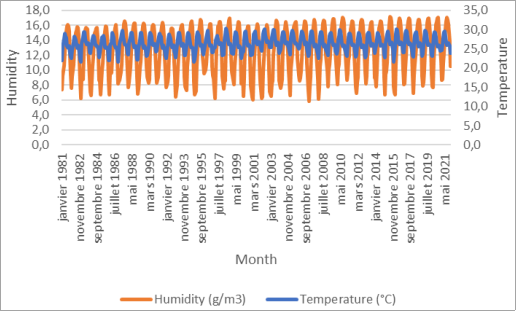
Figure 1. Temperature and humidity trends from 1981 to 2021.
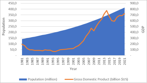
Figure 2. Population and GDP trends, 1981-2021.
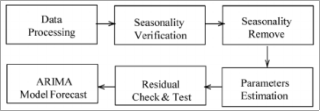
Figure 3. Block diagram of methodology ARIMA model.
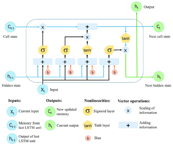
Figure 4. LSTM architecture (Hochreiter & Schmidhuber, 1997).
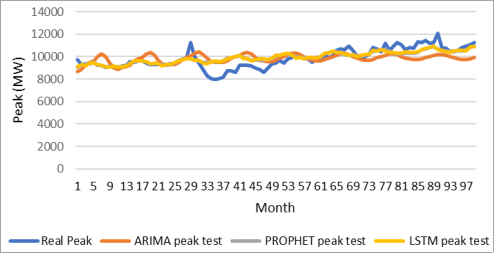
Figure 5. Superpositions of the LSTM, ARIMA and Prophet validation graphs for peak electrical demand.

Figure 6. 2032 WAPP monthly peak electricity demand forecast using Prophet model.
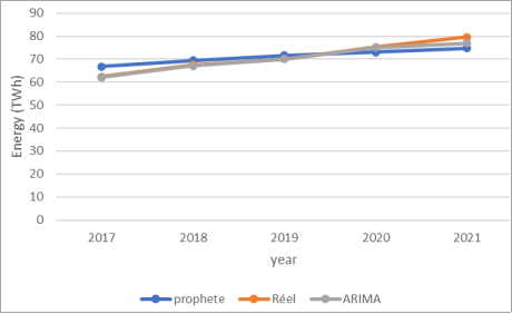
Figure 7. Superpositions of ARIMA and Prophet validation graphs for electricity consumption.
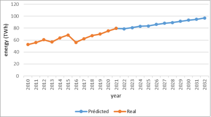
Figure 8. Electricity consumption forecast for 2032 using ARIMA model.
Information