6. Theoretical Background
Modern portfolio theory provides the conceptual basis for risk–return optimization. Markowitz
| [12] | Markowitz, H. M. (1952), “Portfolio Selection”, The Journal of Finance, Vol. 7, No. 1, pp. 77–91. |
| [13] | Markowitz, H. (1959), Portfolio Selection: Efficient Diversification of Investments, Basil Blackwell, New York. |
[12, 13]
established that diversification can minimize total portfolio variance through combining assets with imperfectly correlated returns. Sharpe
| [25] | Sharpe, W. F. (1964), “Capital Asset Prices: A Theory of Market Equilibrium under Conditions of Risk”, The Journal of Finance, Vol. 19, No. 3, pp. 425–442. |
| [26] | Sharpe, W. F. (1966), “Mutual Fund Performance”, The Journal of Business, Vol. 39, No. 1, pp. 119–138. |
[25, 26]
later developed the Capital Asset Pricing Model (CAPM), linking expected returns to systematic risk via the beta coefficient.
The theoretical foundations of CAPM were further strengthened by equilibrium models developed by Mossin
| [15] | Mossin, J. (1966), “Equilibrium in a Capital Asset Market”, Econometrica, Vol. 34, No. 4, pp. 768–783. |
[15]
and Lintner
| [10] | Lintner, J. (1965), “The Valuation of Risk Assets and the Selection of Risky Investments in Stock Portfolios and Capital Budgets”, Review of Economics and Statistics, Vol. 47, No. 1, pp. 13–37. |
[10]
, which formalized the relationship between expected return and systematic risk in competitive capital markets. Ross
| [21] | Ross, S. A. (1976), “The Arbitrage Theory of Capital Asset Pricing”, Journal of Economic Theory, Vol. 13, No. 3, pp. 341–360. |
[21]
expanded this to a multi-factor Arbitrage Pricing Theory (APT), while Fama
| [4] | Fama, E. F. (1970), “Efficient Capital Markets: A Review of Theory and Empirical Work”, The Journal of Finance, Vol. 25, No. 2, pp. 383–417. |
[4]
introduced the Efficient Market Hypothesis (EMH), asserting that prices reflect available information in varying degrees of efficiency.
These theories collectively emphasize diversification, efficiency, and rational investor behavior—principles that remain integral to modern portfolio optimization models.
6.1. Modern Portfolio Theory (MPT)
MPT aims to maximize expected return for a given level of risk or minimize risk for a target return. It assumes investors are risk-averse and markets are efficient. Portfolio return is modeled as a weighted average of asset returns, while risk is measured by standard deviation or variance. The theory’s enduring contribution lies in its demonstration that diversification reduces unsystematic risk and allows investors to achieve optimal portfolios along the efficient frontier.
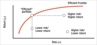
6.2. The Efficient Frontier
The efficient frontier represents the set of portfolios yielding the highest expected return for each risk level or the lowest risk for each expected return. Points below the frontier denote inefficiency; points above are unattainable. The optimal portfolio lies on the frontier at the highest slope of the risk–return curve, indicating maximum return per unit of risk. This concept underpins all subsequent computational and heuristic portfolio optimization models, including the hybrid HGA–AHP approach employed in this study.
Figure 1. Efficient Frontier Curve.
6.2.1. Efficient Frontier (Condensed and Refined)
The efficient frontier represents the set of portfolios that deliver the optimal combination of risk and return. Each point along the curve corresponds to a portfolio that maximizes expected return for a given level of risk or minimizes risk for a target return Markowitz
| [12] | Markowitz, H. M. (1952), “Portfolio Selection”, The Journal of Finance, Vol. 7, No. 1, pp. 77–91. |
| [13] | Markowitz, H. (1959), Portfolio Selection: Efficient Diversification of Investments, Basil Blackwell, New York. |
[12, 13]
. Moving from the lower left to the upper right, both risk and return increase. Achieving an efficient portfolio requires optimized asset weights—random allocation cannot yield efficiency.
De Bondt and Thaler
| [3] | De Bondt, W. F. M. and Thaler, R. (1985), “Does the Stock Market Overreact?”, The Journal of Finance, Vol. 40, No. 3, pp. 793–805. |
[3]
emphasized that each asset contributes a defined proportion to the tangent (optimal) portfolio. For any desired return, there exists a portfolio with the minimum achievable risk, and vice versa. Portfolios on the upper segment of the frontier are efficient
| [11] | Maginn, J. L., Tuttle, D. L., McLeavey, D. W. and Pinto, J. E. (1990), Managing Investment Portfolios: A Dynamic Process, 2nd ed., Warren, Gorham & Lamont. |
[11]
. As market conditions shift, portfolio weights must be periodically rebalanced to maintain efficiency. Markowitz
| [14] | Markowitz, H. M. (1991), “Foundations of Portfolio Theory”, The Journal of Finance, Vol. 46, No. 2, pp. 469–477. |
[14]
and Hagstrom
| [16] | Papahristodoulou, C. and Dotzauer, E. (2004), “Optimal Portfolios Using Linear Programming Models”, Journal of the Operational Research Society, Vol. 55, No. 11, pp. 1169–1177. |
[16]
underscore that maintaining alignment with an investor’s risk tolerance is central to avoiding inefficiency.
6.2.2. Optimal Portfolio Selection
Investors are generally risk-averse; given equal expected returns, they prefer the asset with lower risk
| [11] | Maginn, J. L., Tuttle, D. L., McLeavey, D. W. and Pinto, J. E. (1990), Managing Investment Portfolios: A Dynamic Process, 2nd ed., Warren, Gorham & Lamont. |
[11]
. Hence, a positive relationship exists between expected return and risk
| [18] | Peavy, J. (1990), Cases in Portfolio Management, Association for Investment Management and Research, Charlottesville, VA. |
[18]
. Markowitz
| [12] | Markowitz, H. M. (1952), “Portfolio Selection”, The Journal of Finance, Vol. 7, No. 1, pp. 77–91. |
[12]
defined portfolio return as the weighted average of individual asset returns, while portfolio risk depends on both individual variances and covariances among assets. Diversifying across assets with low or negative correlations minimizes total risk without lowering returns
| [13] | Markowitz, H. (1959), Portfolio Selection: Efficient Diversification of Investments, Basil Blackwell, New York. |
[13]
.
The efficient frontier forms the boundary of optimal portfolios. The
optimal portfolio lies at the tangency point between the frontier and the investor’s highest utility curve
| [3] | De Bondt, W. F. M. and Thaler, R. (1985), “Does the Stock Market Overreact?”, The Journal of Finance, Vol. 40, No. 3, pp. 793–805. |
[3]
reflecting each investor’s unique risk preferences. With the inclusion of a risk-free asset, the Capital Market Line (CML) is formed, representing combinations of risky and risk-free assets
| [6] | Haugen, R. A. (2001), Modern Investment Theory, 5th ed., Prentice Hall, New Jersey. |
[6]
. The tangent portfolio on the CML, known as the market portfolio, comprises all risky assets weighted by market value.
The Security Market Line (SML) extends this framework by relating expected return to systematic risk (beta), as proposed in the CAPM. Beta measures an asset’s covariance with the market portfolio
| [10] | Lintner, J. (1965), “The Valuation of Risk Assets and the Selection of Risky Investments in Stock Portfolios and Capital Budgets”, Review of Economics and Statistics, Vol. 47, No. 1, pp. 13–37. |
[10]
. A higher beta implies higher expected returns. Empirical evidence confirms the relative stability of portfolio betas when sufficient data exists. However, Fama and French
| [5] | Fama, E. F. (1991), “Efficient Capital Markets II”, The Journal of Finance, Vol. 46, No. 5, pp. 1575–1617. |
[5]
found that firm size and book-to-market ratios also explain return variation, suggesting the need to incorporate multiple risk factors in modern portfolio evaluation.
6.3. Measuring Portfolio Performance
6.3.1. Sharpe Ratio
The Sharpe Ratio measures excess return per unit of total risk
| [25] | Sharpe, W. F. (1964), “Capital Asset Prices: A Theory of Market Equilibrium under Conditions of Risk”, The Journal of Finance, Vol. 19, No. 3, pp. 425–442. |
[25]
:
where is the asset return, the risk-free rate, and the standard deviation of excess returns. A higher Sharpe ratio indicates better risk-adjusted performance, making it suitable for comparing portfolios with differing total risks.
6.3.2. Treynor Ratio
The Treynor Ratio assesses excess return relative to systematic risk
| [29] | Treynor, J. L. (1965), “How to Rate Management of Investment Funds”, Harvard Business Review, Vol. 43, No. 1, pp. 63–75. |
[29]
:
where is portfolio return, the risk-free rate, and the portfolio beta. It is most useful for well-diversified portfolios where unsystematic risk is minimal.
6.3.3. Jensen’s Alpha
Jensen’s Alpha measures a portfolio’s abnormal return beyond the CAPM prediction
| [8] | Jensen, M. C. (1968), “The Performance of Mutual Funds in the Period 1945–1964”, The Journal of Finance, Vol. 23, No. 2, pp. 389–416. |
[8]
:
A positive alpha indicates superior risk-adjusted performance, reflecting the manager’s ability to generate returns above market expectations.
6.4. Hybrid Genetic Algorithms (HGA)
Hybrid Genetic Algorithms (HGAs) are evolutionary optimization tools that combine genetic algorithms with local search heuristics
| [6] | Haugen, R. A. (2001), Modern Investment Theory, 5th ed., Prentice Hall, New Jersey. |
[6]
. They are particularly effective for complex, nonlinear, and multi-objective problems, such as portfolio optimization
| [11] | Maginn, J. L., Tuttle, D. L., McLeavey, D. W. and Pinto, J. E. (1990), Managing Investment Portfolios: A Dynamic Process, 2nd ed., Warren, Gorham & Lamont. |
[11]
. HGAs operate on a population of potential solutions, applying selection, crossover, and mutation to evolve toward optimal outcomes. Previous studies have demonstrated that heuristic and evolutionary techniques outperform classical optimization approaches when covariance matrices are singular or highly unstable (Pappas et al.
| [17] | Pappas, D., Kiriakopoulos, K. and Kaimakamis, G. (2010), “Optimal Portfolio Selection with Singular Covariance Matrix”, International Mathematical Forum, Vol. 5, No. 47, pp. 2305–2318. |
[17]
; Sahu et al.
| [22] | Sahu, R., Jain, M. and Garg, G. (2006), “Optimal Portfolio Allocation Using Portfolio Theory and Heuristics Driven Evolutionary Technique”, Journal of Advances in Management Research, Vol. 3, No. 2, pp. 81–87. |
[22]
).
Key advantages include:
1) No requirement for derivative information.
2) Compatibility with nonlinear and mixed-variable models.
3) Global search capability that avoids local optima.
4) Flexibility to integrate domain-specific heuristics.
These features make HGAs ideal for constructing efficient portfolios in markets characterized by high data complexity. These features make HGAs ideal for constructing efficient portfolios in markets characterized by high data complexity
| [24] | Saaty, R. W. (1987), “The Analytic Hierarchy Process—What It Is and How It Is Used”, Mathematical Modelling, Vol. 9, No. 3–5, pp. 161–176. |
[24]
.
6.5. Analytic Hierarchy Process (AHP)
Developed by Saaty
| [23] | Saaty, T. L. (1980), The Analytic Hierarchy Process, McGraw-Hill, New York. |
[23]
, the Analytic Hierarchy Process (AHP) is a structured multi-criteria decision-making method that has been widely applied in financial evaluation and selection problems (Isiklar and Büyüközkan
| [7] | Isiklar, G. and Büyüközkan, G. (2007), “Using a Multi-Criteria Decision-Making Approach to Evaluate Mobile Phone Alternatives”, Computer Standards & Interfaces, Vol. 29, No. 2, pp. 265–274. |
[7]
).
AHP Steps:
1) Define decision hierarchy (goal → criteria → alternatives).
2) Conduct pairwise comparisons using Saaty’s scale.
3) Compute priority weights.
4) Assess consistency using the Consistency Index (CI = (λ_max – N)/(N – 1)); acceptable CI ≤ 0.10.
5) Normalize matrices to derive relative priorities.
6) Aggregate weights to identify the highest-scoring (optimal) alternative.
AHP effectively integrates quantitative and qualitative factors, making it suitable for investment decisions involving multiple, often conflicting objectives
| [2] | Chyi, L. L., Robinson, J. and Reed, R. (2008), “Downside Beta and the Cross-Sectional Determinants of Listed Property Trust Returns”, Journal of Real Estate Portfolio Management, Vol. 14, No. 1, pp. 49–62. |
[2]
.
8. Data Analysis and Results
The study utilizes C#.NET (Visual Studio 2010) to automate the generation, evaluation, and ranking of portfolios. Using daily returns from ASE-listed firms, the algorithm produced 10,000 candidate six-stock portfolios, evaluated their risk–return profiles, and identified the efficient frontier. AHP subsequently selected the optimal portfolio based on the predefined evaluation criteria.
Study Questions
1) Can HGA and AHP jointly identify and select the optimal portfolio?
2) Can HGA effectively construct an efficient frontier for ASE-listed stocks?
3) Does AHP provide a consistent ranking framework for portfolio optimization?
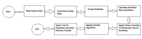
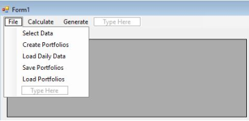
Figure 2. Flowchart of the Implementation Process.
8.1. Implementation Details
The study gathered the stocks data from Amman Stock Exchange website for the year 2015 and used the data to create excel sheets and notepad files.
As
Figure 2 shows, using the file menu and clicking the “Select Data” option, the program will open a select file dialog which allows us to select the stocks data from a notepad (.txt) file.
Figure 3. Creating a File and Selecting Data Using C#.
Data Loading, Encoding, and Portfolio Generation
1) Stock objects. For each ASE-listed firm, the program creates a stock object with:
(i) unique Stock ID, (ii) Stock Code, (iii) expected Return, (iv) Risk, and (v) Daily Returns array.
2) ID scheme and weighting logic. Stocks are assigned integer IDs 60–120 (higher ID ↔ higher expected return). When initializing six-asset portfolios with weights proportional to IDs, this range prevents dominance by a single asset and avoids negligible weights:
Max weight (≈27.9%) if the set includes IDs {120, 60, 61, 62, 63, 64}: .
Min weight (≈9.2%) if the set includes IDs {60, 116, 117, 118, 119, 120}: .
Using 1–60 would yield extreme weights (≈80% vs. ≈0.34%), which is undesirable for balanced portfolio evaluation.
3) Data ingestion. The system parses the prepared text files and loads each stock’s daily returns into the corresponding object; these series are used to compute portfolio-level statistics.
4) Portfolio universe. From the 60 stocks, the algorithm randomly samples without replacement to form 10,000 candidate portfolios, each containing six distinct stocks. Initial weights are set via the ID-proportional rule (later refined by the genetic operators).
5) Risk–return computation. For every candidate portfolio, the program computes expected return (weighted average of component returns) and risk (standard deviation using the full covariance matrix from daily returns). These outputs feed the fitness function used by the HGA.
Figure 4. Calculate Risk and Return.
8.2. Portfolio Risk and Return Calculation (Refined)
When the “Portfolio Risk and Return” option is executed, the program computes each portfolio’s expected return and total risk as follows:
Portfolio Return
(3)
Where:
W: The weight of each stock in the portfolio.
R: The rate of return of each stock in the portfolio.
The weight for each stock in the portfolio is calculated by dividing the asset ID over the summation of the total asset’s IDs of the portfolio.
The 6-asset portfolio risk will be calculated according to the following formula (
6):
(4)
And
To calculate the covariance, we used the stocks daily data to calculate the mean and variance for each stock and followed the following formula to calculate the covariance between each two stocks in any portfolio:
Where:
and: are the sample means return averages.
: is the sample size.
After we calculate the risk and return for each portfolio, we apply the following fitness function to calculate the fitness factor for each portfolio
| [27] | Solimanpur, M., Mansourfar, G. and Ghayour, F. (2015), “Optimum Portfolio Selection Using a Hybrid Genetic Algorithm and Analytic Hierarchy Process”, Studies in Economics and Finance, Vol. 32, No. 3, pp. 379–394. |
[27]
:
(6)
Where:
: is the fitness value of chromosomein direction .
: is the normalized value of return of chromosome .
: is the normalized value of risk of chromosome .
: is the weight of return in direction .
: is the weight of risk in direction .
To produce our results, we used the following weights for risk and return:
Table 1. Summarizes the selected weight coefficients used in the study for calculating the final portfolio fitness values. This streamlined process allows efficient evaluation of 10,000 generated portfolios, facilitating the identification of those lying on the efficient frontier for subsequent AHP ranking.
Weight of risk | Weight of return |
50% | 50% |
40% | 60% |
80% | 20% |
20% | 80% |
60% | 40% |
After we calculate the fitness value for each portfolio, we select the top 10 portfolios based on the highest fitness value.
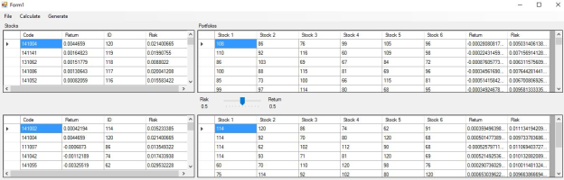
Figure 5. Portfolios and Stocks.
Data Visualization and Portfolio Selection
Figure 5. summarizes the dataset used for optimization.
1) The top-left grid displays stock characteristics (ID, code, return, and risk).
2) The top-right grid lists the 10,000 generated portfolios.
3) The bottom grid presents the top 10 portfolios with their constituent stocks, expected returns, and risks.
HGA Encoding and Evolution Process
Each portfolio is modeled as a gene comprising six chromosomes, each representing one stock. For example, a portfolio containing stocks {114, 120, 86, 74, 62, 91} is encoded in binary form, where each seven-bit sequence corresponds to a stock’s ID. This encoding enables efficient application of genetic operators.
Crossover and Second Generation
The Hybrid Genetic Algorithm operates by recombining the chromosomes of the top 10 portfolios to produce a new generation. In the crossover phase, high-performing genes exchange components to create superior offspring portfolios. The algorithm generates six times the number of parent portfolios, forming the second-generation population.
Selection and Efficient Frontier Construction
After evaluating the second-generation portfolios using the predefined fitness function, the top 10 portfolios are retained. These are plotted on the efficient frontier, illustrating the optimal trade-off between risk and return, as shown in Figure
| [6] | Haugen, R. A. (2001), Modern Investment Theory, 5th ed., Prentice Hall, New Jersey. |
[6]
.
This evolutionary process enhances portfolio performance by iteratively combining the most efficient asset sets until convergence toward the frontier is achieved.
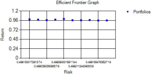
Figure 6. Efficient Frontier.
As shown in
Figure 6, each point on the graph represents one of the top 10 portfolios ranked by the fitness function. Portfolios positioned along the upper boundary satisfy the efficient frontier condition—offering maximum return for a given level of risk. These optimal portfolios are examined further in the results section.
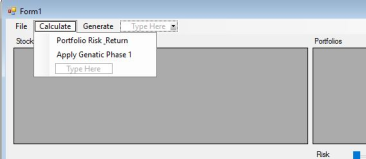
The application was developed to automate the Hybrid Genetic Algorithm (HGA) workflow. Its interface, illustrated in
Figure 5. comprises:
1) Three menus for loading data, calculating portfolio metrics, and managing HGA operations.
2) Five grid views displaying stock data, generated portfolios, top-performing portfolios, and detailed results.
3) A graphical panel for plotting the efficient frontier.
4) A navigation bar for adjusting the weights of risk and return in the fitness function.
This structure allows seamless integration between data visualization, computational modules, and genetic operations—enabling users to perform portfolio optimization, view results dynamically, and refine risk–return preferences within a single interactive environment.
Figure 7. Program Interface.
The program interface organizes data and results across multiple grid views to manage the portfolio optimization process efficiently:
1) Top-left grid: Displays all available stocks retrieved from the Amman Stock Exchange data.
2) Bottom-left grid: Lists the selected stocks that compose the top-performing portfolios used in the HGA to generate second-generation portfolios.
3) Top-right grid: Shows the 10,000 initial portfolios, each containing six randomly selected stocks.
4) Middle-right grid: Displays the top (optimal) portfolios derived from the first-generation evaluation.
5) Bottom-right grid: Presents the second-generation portfolios produced through the HGA crossover process.
As shown in
Figure 6, the interface provides five main control options to execute data loading, portfolio generation, risk–return calculation, HGA crossover, and visualization of the efficient frontier. This modular structure ensures smooth workflow execution and clear visualization of every optimization stage.
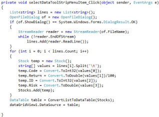
Figure 8 shows the code executed when the “Select Data” option is clicked from the file menu. The first line defines a list named lines to store the data. The second line creates and displays an open file dialog box, allowing the user to select a txt file containing the stock data.
Figure 9. Select Data Code.
The “IF statement” block is used to make sure a file is selected and then add the file lines into the list of lines which we defined in the first line.
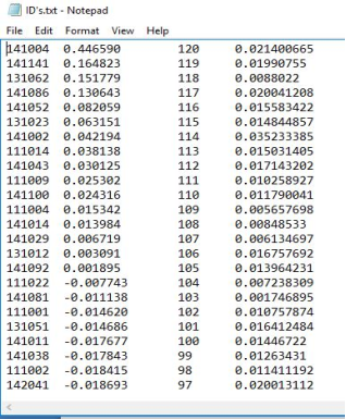
Figure 9. shows the stocks data file. Each line in the file represents a stock where the entries represent the stock code, expected return, ID and risk respectively. The entries are
Figure 10. Stocks Data File.
The “For loop” creates a stock object for each line, assigning its code, expected return, ID, and risk before adding it to the stock list. The last two lines display the data in the application’s grid view.
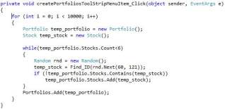
Figure 10. shows the code executed when the “Create Portfolios” option is selected. The function includes a for-loop that repeats the process 10,000 times. It first defines a temporary portfolio and stock, then uses a while-loop to add six stocks to the portfolio. Within the while-loop, a random number generator produces values between 60 and 120. Each generated number is matched to a stock ID, and the corresponding stock is assigned to the temporary stock variable.
Figure 11. Creating Portfolios Code.
The code ensures that each portfolio contains unique stocks, preventing duplicates. When a portfolio reaches six stocks, the while-loop stops adding more. The portfolio is then added to a list, and the process repeats until 10,000 portfolios are created.
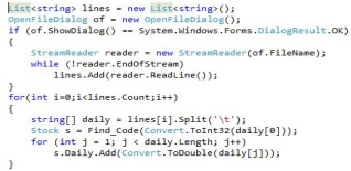
Figure 11 shows the code executed when the “Load Daily Data” option is selected. The first line defines a list named lines to store string values, and the second line creates an open file dialog box to select the file containing the stocks’ daily data.
Figure 12. Load Daily Data Code.
The if-statement ensures a file is selected before reading its contents and storing them in the lines array. In the for-loop, each line is split by tab spaces into an array named daily. The code then locates the stock with the matching code from the selected file, and the inner for-loop adds its daily data to the stock.
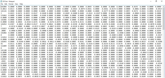
Figure 13shows the daily data file, where each line represents a stock. Each line begins with the stock code, followed by its daily returns, separated by tabs.
Figure 13. Daily Data File.
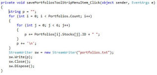
Figure 13 shows the code executed when the “Save Portfolios” option is selected. Because creating 10,000 portfolios is time-consuming, requiring repeated random ID generation, stock searches, and duplication checks, the portfolios are created once and then saved for later use to ensure consistent results. The function saves each portfolio’s stock IDs as a string and writes them to a file named “portfolios.txt.”
Figure 14. Save Portfolios Code.
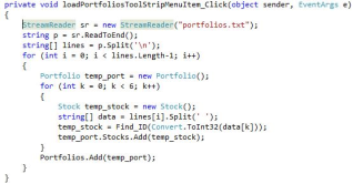
Figure 13 shows the code executed when the “Load Portfolios” option is selected. The code creates a file reader to read the contents of “portfolios.txt” and uses the saved stock IDs to recreate the portfolios.
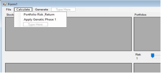
Figure 15. Calculate Menu Options.
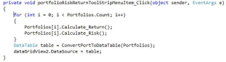
Figure 15 shows the code which is used to calculate the risk and return for each portfolio, as we can see in the figure, the code calls the functions from the portfolio class to calculate the risk and return.
Figure 16. Calculate Risk and Return Code.
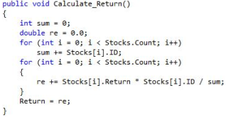
Figure 16 shows the code used to calculate portfolio return. A variable named sum is defined to store the total of all stock IDs, which is then used to calculate each stock’s weight (stock ID ÷ total ID sum). In the second for-loop, each stock’s return is multiplied by its weight and added to the variable re. Finally, the function returns the portfolio’s expected return.
Figure 17. Calculate Return Code.
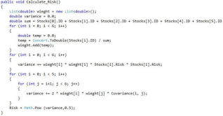
Figure 17 shows the code used to calculate portfolio risk. To simplify the equation, it is divided into three loops. The first for-loop calculates each stock’s weight and stores it in a list for easy access. The second loop calculates the terms containing the square of the weight multiplied by the square of the stock’s risk and adds them to the variable variance, as shown in Equation (
5). The final for-loop calculates the terms requiring covariance by calling the Covariance (i, j) function, which computes the covariance between stocks
i and
j.
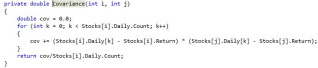
Figure 18. Calculate Risk Code.
Figure 18 shows the code used to calculate the covariance between two stocks. Inside the for-loop, the difference between each stock’s daily value and its expected return is calculated, multiplied together, and added to the variable cov. This process repeats all available daily data. Finally, the function divides cov by the number of data points and returns the result as the covariance between stocks
i and
j.
Figure 19. Covariance Code.
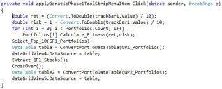
Figure 19 shows the code for applying HGA and crossover operation. The first line reads the return weight from the application’s track bar, and the second calculates the corresponding risk weight. The for-loop then computes the fitness of each portfolio based on the selected risk and returns weights.
Figure 20. Calculate Menu Options.
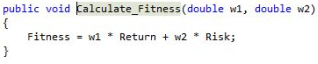
Figure 20 shows the fitness calculation code, which multiplies the return weight by the portfolio’s expected return and adds it to the product of the risk weight and the portfolio’s expected risk. The function Select_Top_10 is then called, passing the portfolio list GP1_Portfolios to store the top 10 portfolios.
Figure 21. Calculate Fitness Code.
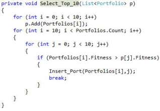
Figure 21 shows the code for selecting the top 10 portfolios. In the first for-loop, the initial 10 portfolios are added to the list. The second loop compares each portfolio’s fitness with those of the top 10; if a portfolio has higher fitness, it replaces the lower one, and the loop breaks to prevent multiple replacements. The following two lines format and display the data in the grid view. Finally, the functions Extract_GP1_Stocks and Crossover are called.
Figure 22. Select Top 10 Portfolios Code.
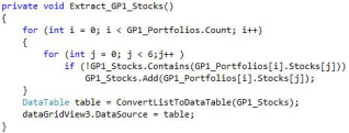
Figure 22 shows the code used to extract GP1 stocks. GP1 is the list containing the top 10 portfolios with the highest fitness. This function extracts the stocks used to form these portfolios, which serve as genes for the upcoming crossover operation. The function checks whether each stock is already in the GP1_Stocks list; if not, it adds it and updates the grid view in the application interface.
Figure 23. Extract GP1 Stocks Code.
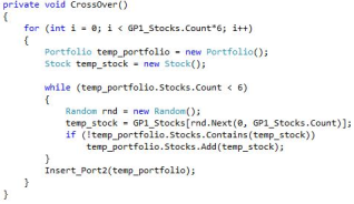
Figure 23 shows the code for the crossover operation, the core function of the HGA. The crossover swaps genes between the best-performing chromosomes to generate improved ones. Instead of swapping single genes, the Extract_GP1_Stocks function creates a gene pool used to form a new generation of portfolios. The function creates temporary portfolio and stock objects, generates a random number within the range of extracted stocks, and adds the selected stock to the portfolio after ensuring it is unique. It also checks that each new portfolio is distinct. This process repeats until six times the number of extracted stocks are generated, after which Genetic Phase 2 is applied, and the top 10 portfolios are selected.
Figure 24. Crossover Code.
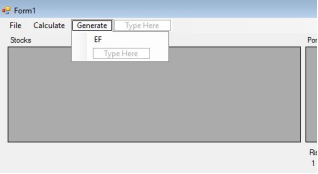
Figure 24 shows the Generate menu, which includes a single option to create the efficient frontier graph displayed in the bottom-left section of the application interface. It’s important to note that the portfolio risk and return values must be normalized before generating the efficient frontier graph.
Figure 25. Generate Menu.
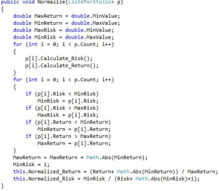
Figure 26. Normalization Code.
Figure 26 shows the code used to normalize each portfolio’s risk and return values. The normalized return is calculated by dividing the portfolio’s return by the maximum return, while the normalized risk is obtained by dividing the minimum risk by the portfolio’s expected risk. To achieve this, the code first identifies the maximum and minimum risk and return values, then shifts the intervals to positive ranges to avoid division-by-zero errors before calculating the normalized values.
8.3. Results Obtained Using the Hybrid Genetic Algorithm
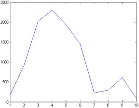
After explaining how the code works, this section presents the program’s results. Figure 27 shows the histogram of the 10,000 portfolios’ expected returns, where the Y-axis represents frequency and the X-axis represents the expected return multiplied by 100. The histogram illustrates the distribution of portfolio expected returns.
Figure 27. Return Histogram.
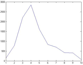
Figure 28 shows the histogram of the 10,000 portfolios’ risks, where the Y-axis represents frequency and the X-axis represents risk multiplied by 100. The histogram illustrates the distribution of portfolio risks.
Figure 28. Risk Histogram.
To obtain the results, five different tests were conducted, each using different risk and return weights in the portfolio fitness calculation. The test with weights of 0.5 – 0.5 is presented here, while the others are included in 1.
0.5 – 0.5 Risk & Return Weights.
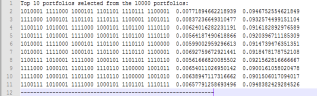
In this test, equal weights of 0.5 were assigned to both risk and return in the fitness function. Using these weights, the top 10 portfolios were selected from the 10,000 generated portfolios based on their fitness scores.
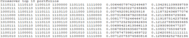
Figure 29. shows the top 10 portfolios. The first six segments represent the portfolio’s chromosomes, each corresponding to a stock. The last two segments indicate the portfolio’s risk and return. Each chromosome is converted into its decimal equivalent, representing the stock ID, which is then used to calculate the stock’s weight in the portfolio.
Figure 29. Top 10 Portfolios Selected from the 10,000 Portfolios.
For example, let’s consider the first portfolio shown in
Figure 29. The portfolio chromosome is [1010001 1111000 1000101 1101101 1110111 1100001], consisting of six genes. When each gene is converted to its decimal equivalent, the stock IDs are (81, 120, 69, 109, 119, 97). The weights for each stock are then calculated as follows (Solimanpur, 2020):
The share of each company in this portfolio is obtained as follows
| [27] | Solimanpur, M., Mansourfar, G. and Ghayour, F. (2015), “Optimum Portfolio Selection Using a Hybrid Genetic Algorithm and Analytic Hierarchy Process”, Studies in Economics and Finance, Vol. 32, No. 3, pp. 379–394. |
[27]
.
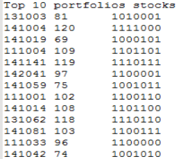
The top 10 portfolios are then used to extract the genes for the crossover operation.
Figure 30. shows the genes and corresponding stocks extracted from these portfolios. Using these genes, the crossover operation generates the second generation of portfolios, from which the top 10 are selected based on the fitness function.
Figure 30. Genes and Stocks used to Create Top 10 Portfolios.
Figure 30 shows the top 10 portfolios of crossover results. These portfolios are used to draw the efficient frontier graph.
Figure 31. Top 10 Second Generation Portfolios.
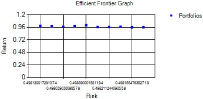
Figure 32. Efficient Frontier Graph.
The proposed HGA was implemented in C# and applied to data from the Amman Stock Exchange for the year 2015. Using HGA to solve Markowitz’s portfolio optimization problem, 10 optimal portfolios were obtained.
Figure 32. shows the efficient frontier generated by the proposed HGA. The annual returns of the optimal portfolios range from 10.552% to 13.429%, while their risks range from 0.646% to 0.818%. The next section introduces an AHP-based decision-making technique to help select the most suitable portfolio among the 10 options.
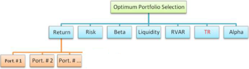
8.4. Portfolio Selection via Analytic Hierarchy Process
Figure 33. Proposed Hierarchy of the Portfolio Selection Problem.
Figure 33 illustrates the proposed hierarchical structure for the optimal portfolio selection problem, including the alternatives obtained through HGA and the identified criteria. The decision hierarchy has three levels: the top level (Level 1) represents the main objective—optimal portfolio selection; the second level includes the seven criteria: return, risk, beta ratio, liquidity, RVAR, TR, and alpha ratio; and the bottom level (Level 3) lists the 10 portfolios generated by HGA as the decision alternatives. The optimal portfolio is portfolio number 8
| [30] | Vargas, L. G. (1990), “An Overview of the Analytic Hierarchy Process and Its Applications”, European Journal of Operational Research, Vol. 48, No. 1, pp. 2–8. |
[30]
.
Table 2 presents the top 10 portfolios generated by the GA operation along with their corresponding criteria. It is also noted that the Sharpe and Treynor ratios for the market portfolio were -8.646 and -0.038049125, respectively.
Table 2. Seven Criteria's Portfolios.
Por.# | Risk | Return | liquidity | Sharpe | Beta | TR | Alpha |
1 | 0.646% | 13.429% | 1.702 | 14.904 | 0.153 | 0.631 | 0.102 |
2 | 0.676% | 12.927% | 1.815 | 13.512 | 0.191 | 0.478 | 0.099 |
3 | 0.745% | 11.873% | 2.159 | 10.834 | 0.197 | 0.410 | 0.088 |
4 | 0.732% | 12.120% | 2.462 | 11.368 | 0.295 | 0.282 | 0.094 |
5 | 0.818% | 11.919% | 2.301 | 9.928 | 0.146 | 0.554 | 0.087 |
6 | 0.707% | 12.123% | 2.018 | 11.768 | 0.281 | 0.296 | 0.094 |
7 | 0.695% | 12.931% | 1.913 | 13.130 | 0.211 | 0.434 | 0.099 |
8 | 0.679% | 10.552% | 0.860 | 9.950 | 0.133 | 0.507 | 0.073 |
9 | 0.787% | 12.620% | 1.966 | 11.201 | 0.335 | 0.263 | 0.101 |
10 | 0.712% | 12.591% | 1.843 | 12.345 | 0.166 | 0.529 | 0.094 |
Table 2. shows the results of the hierarchy analysis process, where the Y-axis represents the portfolio number and the X-axis represents the portfolio’s relative preference weight. As shown, the optimal portfolio is portfolio number 8.
Figure 34. Portfolio Hierarchy Analysis.
Therefore, the portfolios can be displayed according to their optimality as in the following
Table 3:
Table 3. Portfolios Optimality.
Portfolio # | Optimality Order |
1 | 2 |
2 | 7 |
3 | 7 |
4 | 6 |
5 | 3 |
6 | 5 |
7 | 7 |
8 | 1 |
9 | 7 |
10 | 4 |
8.5. Summary of the Section
This section outlines the HGA implementation process, the results obtained, and portfolio selection using AHP. The next section presents the study’s summary, conclusions, and recommendations for future research.
Section Six.