Dielectric Relaxation and Electrical Modulus Formalism in Solids

Mrityunjay Kumar

doi:doi:10.11648/j.ep.20260901.11

Research Article |

| Peer-Reviewed

Dielectric Relaxation and Electrical Modulus Formalism in Solids

Mrityunjay Kumar^*

Published in Engineering Physics (Volume 9, Issue 1)

Received: 6 March 2026 Accepted: 20 March 2026 Published: 13 May 2026

Views: Downloads:

Download PDF

Share This Article

Twitter
Linked In
Facebook

Abstract

The dielectric relaxation effects give a very important understanding of the microscopic dynamics of dipoles and charge carriers in solids, especially those materials where disorder, conductivity and interfacial effects make the dielectric response difficult to understand. A single and pedagogic exposition of dielectric relaxation in this work is introduced, starting with the analogous time domain Debye polarization equation and moving stepwise to the frequency domain complex permittivity formulation. Real and complex values of the dielectric permittivity are obtained and their physical interpretation, loss peak performance and Cole Cole presentation are provided in details. Abnormal Debye behaviour in real solids is treated by the Cole-Cole, Cole-Davidson and Havriliak-Negami models, which are focused on the characteristics of describing distributed and asymmetric relaxation-time spectra. In order to by-pass the restrictions due to the conductivity of the dc and as polarization of the electrodes at low frequencies, electrical modulus formalism is presented and derived in the case of Debye and non-Debye relaxation model. The usefulness of this method is illustrated by the fact that the complex modulus spectra of Nd₂FeTiO₆ ceramic were analyzed in the entire span of temperatures. The presence of depressed and asymmetric modulus arcs, scaled master-curve behavior also obviously signal non-Debye relaxation behavior best fitted by the HavriliakNegami model. The joint analysis of permittivity-modulus offers a powerful model of isolating the intrinsic bulk relaxation and extrinsic conductive sources, and can be used to obtain physically useful relaxation parameters. The work is not only an introduction on a tutorial level, but also a practical guide to researchers working on dielectric and impedance spectroscopy of solid materials.

Published in	Engineering Physics (Volume 9, Issue 1)
DOI	10.11648/j.ep.20260901.11
Page(s)	1-9
Creative Commons	This is an Open Access article, distributed under the terms of the Creative Commons Attribution 4.0 International License (http://creativecommons.org/licenses/by/4.0/), which permits unrestricted use, distribution and reproduction in any medium or format, provided the original work is properly cited.
Copyright	Copyright © The Author(s), 2026. Published by Science Publishing Group

Keywords

Dielectric, Electric Modulus, Relaxation, Polarization, Permittivity

1. Introduction

Dielectric relaxation processes have a central role in condensed-matter physics and materials science as well as applied electromagnetism, and give a direct view to the microscopic dynamics of dipoles and charge carriers in matter. The polarization induced in a dielectric medium when an external electric field is applied to it does not in general follow the field at any moment

[1-4]

. Rather, both temperature and the time scale of the applied field depend on the delayed response due to inertia, intermolecular, and lattice, and energy barriers. This retarded reaction or dielectric relaxation is thus a study that has become very important in studying the mechanisms of motion in liquids, defect and ionic dynamics in solids, and functional behavior in technologically significant materials such as ferroelectrics, polymers, and solid electrolytes

[5]

The most fundamental and historically the most significant theoretical explanation of dielectric relaxation presented in the framework of polar liquids was done by Debye. The Debye picture Permanent dipoles in a viscous medium experience the rotational diffusion and relax to equilibrium with one characteristic time constant. Although the Debye model is based on idealized assumptions, it has been a foundation of the dielectric theory, both as a point of entry into the theory and as a point of reference where more complicated behaviors are examined

[6, 7]

In macroscopic perspective, the Debye method connects the time dependence of the polarization to the force provided using an electric field in a first-order linear equation of change. This equation in its transformed form to the frequency domain is the complex dielectric permittivity, given by which is the complex dielectric permittivity of energy stored and dissipated per cycle of the applied field, the real and imaginary components of which are the energy stored and dissipated, respectively. The appearance of a characteristic loss peak in

ε^{''} (ω)

at a frequency inversely proportional to the relaxation time provides a simple and experimentally accessible signature of relaxation processes. Consequently, dielectric spectroscopy—spanning frequencies from millihertz to terahertz—has become a powerful experimental technique for probing relaxation dynamics across many orders of magnitude in time

[8, 9]

In real substances, ideal Debye behavior is, however, the exception rather than the norm. Relaxation processes in solids and in complex molecular systems are also commonly broadened by structural disorder, cooperative motion, and the multiplicity of microscopic processes. Experimental dielectric spectra often have asymmetric loss curves, depressed semicircles on Cole-Cole curves, or power-law tails in the low-frequency region

[10]

. In order to explain these deviations, some empirical generalizations of the Debye model have been suggested, including the Cole-Cole, Cole-Davidson and Havriliak-Negami functions, which are commonly employed. The models add more parameters that give a better description of the distributions of relaxation times and still have a clear relation to the underlying Debye framework

[11]

Another complication arises from electrical conductivity and electrode polarization, effects that are particularly pronounced in ionic conductors and many ceramic or polymeric solids. At low frequencies, mobile charge carriers can dominate the dielectric response, leading to very large apparent values of the real permittivity and obscuring intrinsic dipolar relaxations. In such cases, direct interpretation of

ε^{'} (ω)

and

ε^{''} (ω)

becomes challenging. To address this issue, the electrical modulus formalism has proven to be a valuable complementary representation. By defining the complex modulus

M^{*} (ω) = 1 / ε^{*} (ω)

, contributions from large permittivity are suppressed, and bulk relaxation processes often emerge more distinctly in the modulus loss

M^{''} (ω)

. The modulus approach has therefore become standard in the analysis of dielectric and impedance spectroscopy data for solid electrolytes, glasses, and disordered solids

[12, 13]

Debye and modulus formalisms give a didactic lesson of how simple physical conjectures can be made into experimentally verifiable predictions. However, in most textbooks and research papers, derivations are either given in a very compressed version or are dispersed in various contexts, such that students and emerging researchers in the field have trouble trying to trace the logical development of basic principles to realistic data analysis processes. A concise, independent exposition, beginning with the time-domain treatment of what polarization is, makes a smooth, logical progression to the frequency-domain response, and then adds the modulus representation, can go a long way to increase both conceptual insight and analytical vigour. The purpose of the current paper is to provide such a logical and pedagogically related exposition. We start by once again considering the expression of the Debye relaxation equation of polarization and obtain the complex dielectric permittivity and its real and imaginary components. Discussed are the physical meaning of the loss peak and the associated geometry of the Cole-Cole plane. Then we introduce the Cole-Cole generalization, which is a very slight extension that describes non-Debye behavior in terms of a distribution of relaxation times. Lastly, we encourage and formulate the electrical modulus formalism and describe its utilitarian benefits in the analysis of dielectric information of solid materials with large conductivity influences.

In the course of the article, the gravitation is given to the derivation clarity, direct interpretation of the physical process, and direct application to the experimental and computational studies. This work will be addressed to both the tutorial level of a student of physics at the university level and also to a concise reference of the researcher involved in dielectric and impedance spectroscopy studies by means of a unified presentation of equations and concepts.

2. Time-domain Description of Dielectric Relaxation

The Debye model describes dielectric relaxation by assuming that the orientational part of the polarization does not respond instantaneously to an applied electric field but relaxes toward equilibrium with a single characteristic time. Let

P (t)

denote the macroscopic polarization associated with this slow process, and let

P_{s} (t)

be the equilibrium polarization corresponding to the instantaneous value of the electric field. The relaxation is modeled by a linear first-order differential equation in which the rate of change of polarization is proportional to the difference between the instantaneous and equilibrium values.

P (t) = P_{s} [1 - \exp (- \frac{t}{τ})]

(1)

The proportionality constant defines the relaxation time

τ

. This simple equation embodies the assumption that the system “forgets” its previous state exponentially in time and that the response is linear in the applied field. When a time-dependent electric field is applied, this equation governs how polarization evolves in time. The time dependence of the electric field (E) and the electric displacement (D) in a dielectric medium can be described by the differential equation.

τ \frac{dD (t)}{dt} + D (t) = τ ε_{0} ε_{\infty} \frac{dE (t)}{dt} + ε_{0} ε_{s} E (t)

(2)

Dielectric spectroscopy experiments are usually performed with sinusoidally varying electric fields

[14]

. For a harmonic field of angular frequency

ω

, the time-domain relaxation equation can be transformed to the frequency domain. Supposing that a time-varying field

E (t) = E_{0} e^{iωt}

is applied to a dielectric, the resulting electric displacement D(t) is given by

D (t) = D_{0} e^{i (ωt - ϕ)}

incorporating these expressions in the above differential equation leads to:

\frac{D (t)}{ε_{0} E (t)} = \frac{ε_{s} + ε_{\infty} (iωt)}{1 + iωt}

(3)

The resulting response is expressed in terms of the complex dielectric permittivity

ε^{*} (ω)

, which contains both the in-phase and out-of-phase components of the polarization response. Employing the relation:

ε^{*} = \frac{D (t)}{ε_{0} E (t)}

(4)

and rearranging the terms in the second part of Eq. (3), the Debye dispersion equation can be written as:

ε^{*} (ω) = ε_{\infty} + \frac{ε_{s} - ε_{\infty}}{1 + iωτ}

(5)

In the Debye model, the complex permittivity has a particularly simple form. It is written as the sum of a high-frequency permittivity

ε_{\infty}

, representing instantaneous electronic and atomic polarization, and a relaxing contribution that depends on the relaxation time

τ

ε^{*} (ω)

is the complex dielectric permittivity defined as

ε^{*} (ω) = ε^{'} (ω) + ε" (ω)

. Separating the complex permittivity into real and imaginary parts provides direct physical insight, the following expressions for the real and imaginary part of dielectric permittivity are obtained.

ε^{' (ω)} = ε_{\infty} + \frac{ε_{s} - ε_{\infty}}{1 + ω^{2} τ^{2}}

(6)

and

ε^{″ (ω)} = \frac{(ε_{s} - ε_{\infty}) ωτ}{1 + ω^{2} τ^{2}}

(7)

where

ω = 2 πf

is the angular frequency of the field. The real part

ε^{'} (ω)

describes the energy stored in the dielectric, while the imaginary part

ε^{''} (ω)

represents energy dissipation or dielectric loss

[15, 16]

. Examining the function

ε ″ (ω)

to find that the maximum dielectric loss occurs at the frequency

ω_{\max} = 1 / τ

and is equal to:

ε ″_{ω_{\max}} = \frac{ε_{s} - ε_{\infty}}{2}

(8)

at the same frequency

ε'

takes the value:

ε'_{ω_{\max}} = \frac{ε_{s} + ε_{\infty}}{2}

(9)

{(ε^{'} - \frac{ε_{s} + ε_{\infty}}{2})}^{2} + {(ε^{″})}^{2} = {(\frac{ε_{s} - ε_{\infty}}{2})}^{2}

(10)

This equation implies that the center of the semicircle lies on the x-axis with coordinates

(\frac{ε_{s} + ε_{\infty}}{2}, 0)

and the radius is

(\frac{ε_{s} - ε_{\infty}}{2})

. The Cole-Cole representation is used to assess the agreement between the Debye equations and experimental data. The difference between the static permittivity

ε_{s}

and

ε_{\infty}

is denoted by

Δ ε

, which measures the strength of the relaxing dipolar contribution.

In the Debye model,

ε^{'} (ω)

decreases smoothly from

ε_{s}

at low frequencies to

ε_{\infty}

at high frequencies, whereas

ε^{''} (ω)

exhibits a well-defined maximum. This loss peak occurs when the angular frequency satisfies

ωτ = 1

, directly linking an experimentally observable quantity to the microscopic relaxation time. A convenient graphical representation of Debye relaxation is the Cole–Cole plot, in which

ε^{''}

is plotted against

ε^{'}

with frequency as an implicit parameter. For an ideal Debye process, this plot is a perfect semicircle centered on the real axis, a geometric signature of a single relaxation time.

3. Cole-Cole, Cole-Davidson, Havriliak-Negami Equations

The Debye dispersion equations describe a dielectric relaxation process characterized by a single relaxation period. While numerous polar liquids align well with these theoretical curves, discrepancies from the dielectric response of solid dielectrics are likely seen. In a solid dielectric medium, several relaxations may occur. These relaxations may result from many types of permanent and induced dipoles.

The Debye model assumes that all relaxing dipoles in a material are characterized by a single relaxation time. While this assumption is adequate for idealized systems, experimental dielectric spectra of real materials frequently display broadened and asymmetric loss peaks, indicating the presence of a distribution of relaxation times rather than a single characteristic value. Such distributions arise from structural disorder, interactions among dipoles, variations in local environments, and cooperative relaxation processes. To account for these deviations from ideal Debye behavior, several empirical generalizations of the Debye relaxation function have been developed.

One of the most widely used extensions is the Cole–Cole (CC) model, which introduces a symmetric broadening of the relaxation spectrum. In this formulation, the complex permittivity is written as

ε^{*} (ω) = ε_{\infty} + \frac{ε_{s} - ε_{\infty}}{1 + {(iωτ)}^{1 - α}}

(11)

where

0 \leq α < 1

is the Cole–Cole parameter. When

α = 0

, the Debye expression is recovered. As

α

increases, the dielectric loss peak becomes broader and the corresponding Cole–Cole plot changes from a perfect semicircle to a depressed arc whose center lies below the real axis. Physically, the parameter

α

reflects a symmetric distribution of relaxation times around the mean value

τ

. Furthermore, the Cole-Cole plot exhibits a semicircle with its centre positioned beneath the x-axis. The Cole-Cole equation represents a series of discrete relaxations, each characterised as a Debye-type process with a singular relaxation time. The various relaxation times are symmetrically distributed around the time τ in Equation (11). The width of relaxation curves is seen as indicative of the interactions between dipoles and their surroundings. By isolating the real and imaginary components of the equation (11), the subsequent equations are obtained

[17]

ε^{'} = ε_{\infty} + \frac{(ε_{s} - ε_{\infty}) [1 + {(ωτ)}^{1 - α} \sin \frac{απ}{2}]}{1 + {(ωτ)}^{2 (1 - α)} + 2 {(ωτ)}^{1 - α} \sin \frac{απ}{2}}

(12)

and

ε^{″} = \frac{(ε_{s} - ε_{\infty}) {(ωτ)}^{1 - α} \cos \frac{απ}{2}}{1 + {(ωτ)}^{2 (1 - α)} + 2 {(ωτ)}^{1 - α} \sin \frac{απ}{2}}

(13)

In many materials, however, the relaxation spectrum exhibits an asymmetric broadening, particularly on the high-frequency side of the loss peak. This behavior is better described by the Cole–Davidson (CD) model, which modifies the Debye response as

ε^{*} (ω) = ε_{\infty} + \frac{ε_{s} - ε_{\infty}}{{(1 + iωτ)}^{γ}}

(14)

where

0 < β \leq 1

. The Cole–Davidson model reduces to the Debye form when

β = 1

. In accordance with the Davidson Cole model, the condition

ω_{\max} τ = 1

is invalid at the maxima of dielectric loss. This is given by

ω_{\max} τ = \tan (\frac{1}{γ + 1} \frac{π}{2})

(15)

In contrast to the Cole–Cole model, the Cole–Davidson function produces an asymmetric loss peak with a long tail extending toward lower frequencies. This asymmetry is often associated with hierarchical or constrained relaxation processes, commonly observed in polymers and glassy systems

[18]

. The real and imaginary part of the dielectric constant is given by

ε^{'} = ε_{\infty} + (ε_{s} - ε_{\infty}) {(\cos ϕ)}^{γ} \cos γϕ

(16)

and

ε^{″} = (ε_{s} - ε_{\infty}) {(\cos ϕ)}^{γ} sinγϕ

(17)

where

\tan ϕ = ωτ

(18)

The most general and flexible empirical description of dielectric relaxation is provided by the Havriliak–Negami (HN) model, which combines the features of both Cole–Cole and Cole–Davidson forms. The complex permittivity in this model is expressed as

ε^{*} (ω) = ε_{\infty} + \frac{ε_{s} - ε_{\infty}}{{[1 + {(iωτ)}^{1 - α}]}^{γ}}

(19)

with

0 \leq α < 1

and

0 < β \leq 1

. The Havriliak–Negami expression reduces to the Cole–Cole model when

β = 1

and to the Cole–Davidson model when

α = 0

. When both parameters are nonzero, the relaxation spectrum exhibits both symmetric and asymmetric broadening, allowing excellent fits to a wide range of experimental dielectric data

[19]

. Separating the real and imaginary parts of the dielectric constant yields.

ε^{'} = ε_{\infty} + \frac{(ε_{s} - ε_{\infty}) \cos γϕ}{[1 + {(ωτ)}^{2 (1 - α)} + 2 {(ωτ)}^{1 - α} \sin \frac{απγ}{2}]}

(20)

and

ε^{″} = \frac{(ε_{s} - ε_{\infty}) \sin γϕ}{[1 + {(ωτ)}^{2 (1 - α)} + 2 {(ωτ)}^{1 - α} \sin \frac{απγ}{2}]}

(21)

According to the Havriliak–Negami (HN) model, the frequency corresponding to the maximum dielectric loss is given by

ω_{\max} = \frac{1}{τ} {[\frac{\sin (\frac{(1 - α) γπ}{2 (1 + γ)})}{\sin (\frac{(1 - α) π}{2 [(1 + γ)]})}]}^{1 / (1 - α)}

(22)

It is important to point out that Eqs. (11), (14), and (19) are semiempirical and don't have a clear theoretical basis. Their validity comes from the fact that they fit experimental data from numerous materials better.

The Cole–Cole, Cole–Davidson and Havriliak–Negami descriptions you have just reviewed make it clear that realistic dielectric spectra are generally composed of overlapping processes with broadened and often asymmetric relaxation-time distributions. These phenomenological forms capture how the complex permittivity

ε^{*} (ω)

departs from the ideal Debye response: loss peaks shift, semicircles become depressed, and high-frequency tails appear. In many experimental situations—particularly for solids, ionic conductors, and disordered materials—however, an additional complication arises. Extrinsic effects such as electrode polarization, space-charge accumulation, and dc conductivity frequently dominate the low-frequency permittivity, producing very large

ε^{'} (ω)

and a

1 / ω

rise in

ε^{''} (ω)

. These features can mask the intrinsic relaxation(s) you have modeled with HN-type functions and make robust extraction of bulk relaxation parameters difficult.

A simple change of perspective often resolves this difficulty. Instead of emphasizing how the material polarizes (the permittivity view), one can emphasize how the internal electric field relaxes. This is the idea behind the electrical modulus formalism. Define the complex electrical modulus as the reciprocal of the complex permittivity,

M^{*} (ω) = \frac{1}{ε^{*} (ω)} = M^{'} (ω) + i M^{''} (ω)

(23)

where, for clarity, we use the convention

ε^{*} (ω) = ε^{'} (ω) - i ε^{''} (ω)

. Algebraically, the modulus components are obtained from the permittivity components by inversion:

M^{'} (ω) = \frac{ε^{'} (ω)}{ε^{'} (ω)^{2} + ε^{''} (ω)^{2}}, M^{''} (ω) = \frac{ε^{''} (ω)}{ε^{'} (ω)^{2} + ε^{''} (ω)^{2}}

(24)

Because very large values of

ε^{'}

(arising from electrode or interfacial polarization) correspond to very small values of

M^{'}

, those extrinsic contributions are strongly suppressed in the modulus representation. In practice this means that a relaxation hidden beneath a conductive background in

ε^{''} (ω)

often appears as a clear peak in

M^{''} (ω)

, making the modulus particularly useful for identifying bulk processes in ionic or poorly conducting solids.

For the single-time Debye model, the modulus can be written explicitly (by algebraic inversion of the Debye

ε^{*} (ω)

) and its loss peak occurs at a frequency shifted from the permittivity peak; this shift depends on the ratio of static to high-frequency permittivity. For non-Debye HN-type relaxations, the same qualitative advantages hold: modulus peaks provide complementary constraints on

τ

and on the breadth/asymmetry parameters you have just discussed. Thus, rather than replacing permittivity analysis, modulus analysis should be used in tandem—fit

ε^{*} (ω)

to quantify dipolar strength and distribution, and examine

M^{*} (ω)

to separate bulk relaxation from interfacial and conductive artefacts.

In the next subsection, we derive

M^{*} (ω)

for Debye, Cole-Cole, Cole-Davison and Havriliak-Negami forms, discuss the relation between the

ε^{''}

and

M^{''}

peak positions, and give practical fitting recipes so that all representations yield consistent, physically meaningful parameters.

The Cole-Cole model:

\begin{matrix} M^{*} = \frac{1}{ε_{r}^{*}} = \frac{1}{ε_{\infty} + \frac{ε_{s} - ε_{\infty}}{1 + (iωτ)^{β}}} = \frac{1}{ε_{\infty}} \cdot \frac{1}{1 + \frac{\frac{ε_{s}}{ε_{\infty}} - 1}{1 + (iωτ)^{β}}} \\ M^{*} & = \frac{1}{ε_{\infty}} [\frac{1 + \frac{ε_{s} / ε_{\infty} - 1}{1 + (iωτ)^{β}} - \frac{ε_{s} / ε_{\infty} - 1}{1 + (iωτ)^{β}}}{1 + \frac{ε_{s} / ε_{\infty} - 1}{1 + (iωτ)^{β}}}] \\ M^{*} & = \frac{1}{ε_{\infty}} [1 - \frac{ε_{s} / ε_{\infty} - 1}{1 + (iωτ)^{β} + ε_{s} / ε_{\infty} - 1}] \\ M^{*} & = \frac{1}{ε_{\infty}} - \frac{\frac{ε_{s}}{ε_{\infty}^{2}} - \frac{1}{ε_{\infty}}}{ε_{s} / ε_{\infty} + (iωτ)^{β}} = \frac{1}{ε_{\infty}} - \frac{\frac{1}{ε_{\infty}} - \frac{1}{ε_{s}}}{1 + (iωτ)^{β} \cdot (\frac{ε_{\infty}}{ε_{s}})} \\ M^{*} & = \frac{1}{ε_{\infty}} - \frac{\frac{1}{ε_{\infty}} - \frac{1}{ε_{s}}}{1 + {(iω τ^{'}_{M})}^{β}} \end{matrix}

M^{*} = M_{\infty} - \frac{M_{\infty} - M_{s}}{1 + {(iω τ^{'}_{M})}^{β}}

(25)

M_{\infty} = 1 / ε_{\infty}

and

M_{s} = 1 / ε_{s}

denote the reciprocal high-frequency and static permittivities, respectively. Furthermore, the relaxation time in the electrical modulus representation,

τ_{M}

, is related to the relaxation time

τ

τ_{M}^{'} = [τ⋅ {(\frac{ε_{\infty}}{ε_{s}})}^{1 / β}] = τ_{M} [{(\frac{ε_{\infty}}{ε_{s}})}^{1 / β - 1}]

(26)

Separating the real and the imaginary parts of equation (25), we get,

M^{'} = M_{\infty} M_{s} \frac{[M_{s} A + (M_{\infty} - M_{s}) \cos ϕ] A}{M_{s}^{2} A^{2} + 2 A (M_{\infty} - M_{s}) M_{s} \cos ϕ + {(M_{\infty} - M_{s})}^{2}}

(27)

M^{″} = M_{\infty} M_{s} \frac{[(M_{\infty} - M_{s}) \sin ϕ] A}{M_{s}^{2} A^{2} + 2 A (M_{\infty} - M_{s}) M_{s} \cos ϕ + {(M_{\infty} - M_{s})}^{2}}

(28)

where

A = {\{1 + 2 {(ωτ)}^{1 - α} \sin \frac{πα}{2} + {(ωτ)}^{2 (1 - α)}\}}^{1 / 2}

(29)

and

φ = \arctan \{\frac{{(ωτ)}^{1 - α} \cos \frac{απ}{2}}{1 + {(ωτ)}^{1 - α} \sin \frac{απ}{2}}\}

(30)

Since the static permittivity

ε_{s}

is always larger than the high-frequency permittivity

ε_{\infty}

, the modulus relaxation time

τ_{M}

is smaller than the permittivity relaxation time

τ

. As a consequence, the peak in the imaginary part of the electrical modulus

M^{''} (ω)

occurs at a higher frequency than the corresponding peak in the dielectric loss

ε^{''} (ω)

[17, 20]

The Cole-Davison:

The modulus can be written compactly as

M^{*} (ω) = M_{\infty} \frac{(1+ iωτ)^{γ}}{(1+ iωτ)^{γ}+ (\frac{M_{\infty}}{M_{s}}− 1)}

(31)

For the Cole–Davidson permittivity function, the corresponding complex electrical modulus yields a response that interpolates between

M_{s}

at low frequencies and

M_{\infty}

at high frequencies and highlights the intrinsic bulk relaxation dynamics

[18]

Separating the real and the imaginary parts of equation (31), we get,

M^{'} = \frac{M_{\infty} M_{s} [M_{s} + (M_{\infty} - M_{s}) {(\cos ϕ)}^{γ} \cos γϕ]}{M_{s}^{2} + (M_{\infty} - M_{s}) {(\cos ϕ)}^{γ} [2 M_{s} \cos γϕ + (M_{\infty} - M_{s}) {(\cos ϕ)}^{γ}]}

(32)

M^{″} = \frac{M_{\infty} M_{s} (M_{\infty} - M_{s}) {(\cos ϕ)}^{γ} \sin γϕ}{M_{s}^{2} + (M_{\infty} - M_{s}) {(\cos ϕ)}^{γ} [2 M_{s} \cos γϕ + (M_{\infty} - M_{s}) {(\cos ϕ)}^{γ}]}

(33)

where

\tan ϕ = ωτ

(34)

and

ω_{\max} τ = \tan (\frac{1}{γ + 1} \frac{π}{2})

(35)

The Havriliak-Negami model:

The corresponding complex electrical modulus becomes

M^{*} (ω) = M_{\infty} \frac{{[1+ {(iωτ)}^{1 - α}]}^{γ}}{{[1+ {(iωτ)}^{1 - α}]}^{γ} + (\frac{M_{\infty}}{M_{s}}− 1)}

(36)

For the Havriliak–Negami permittivity function, the corresponding complex electrical modulus gives a response that evolves from

M_{s}

at low frequencies to

M_{\infty}

at high frequencies and incorporates both symmetric and asymmetric broadening of relaxation times

[19]

. Writing the real and the imaginary parts separately,

M^{'} = M_{\infty} M_{s} \frac{[M_{s} A^{γ} + (M_{\infty} - M_{s}) \cos γϕ] A^{γ}}{M_{s}^{2} A^{2 γ} + 2 A^{γ} (M_{\infty} - M_{s}) M_{s} \cos γϕ + {(M_{\infty} - M_{s})}^{2}}

(37)

M^{″} = M_{\infty} M_{s} \frac{[(M_{\infty} - M_{s}) \sin γϕ] A^{γ}}{M_{s}^{2} A^{2 γ} + 2 A^{γ} (M_{\infty} - M_{s}) M_{s} \cos γϕ + {(M_{\infty} - M_{s})}^{2}}

(38)

4. Application of the Modulus Formalism to Nd₂FeTiO₆ Ceramic

Download: Download full-size image

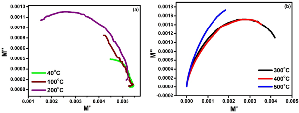
Figure 1. (a) and (b): Plot of real Modulus versus imaginary part of modulus of Nd₂FeTiO₆ceramic.

Figures 1(a) and 1(b) show the complex electric modulus plots (

M^{''}

versus

M^{'}

) at different temperatures of Nd₂FeTiO₆(NFTO) ceramic. Instead of forming perfect semicircular arcs expected for ideal Debye relaxation, the experimental data exhibit depressed and clearly asymmetric arcs, whose centers lie well below the real axis. This deviation from a perfect semicircle confirms the presence of non-Debye relaxation behavior and a distributed spectrum of relaxation times in the material

[21]

. At lower temperatures, the arcs are moderately depressed but already deviate from symmetry, indicating that a simple Cole–Cole (CC) model, which assumes symmetric broadening of relaxation times, is insufficient to describe the data

[22]

. As temperature increases, the asymmetry becomes more pronounced, particularly on the high-frequency side of the arcs, where the curvature changes rapidly, and the arcs appear stretched rather than uniformly broadened. Such behavior cannot be captured adequately by the Cole–Cole model alone.

[17, 21, 22]

The Cole–Davidson (CD) model, which accounts for asymmetric broadening primarily on the high-frequency side, improves the qualitative description but still fails to reproduce the full shape of the arcs over the entire frequency range, especially the combined depression and skewness observed experimentally. This indicates that the relaxation process is governed by both symmetric broadening (distribution width) and asymmetric stretching (non-exponential decay)

[18]

Consequently, the Havriliak–Negami (HN) model provides the most appropriate and comprehensive description of the observed modulus behavior. The HN model incorporates two independent shape parameters, allowing simultaneous control over the degree of arc depression and asymmetry. This flexibility enables it to accurately reproduce the experimental

M^{''}

–

M^{'}

plots across all temperatures. The progressive change in arc shape with temperature further suggests thermally activated relaxation accompanied by a temperature-dependent evolution of the relaxation-time distribution, which is naturally accommodated within the HN formalism. Thus, based on the depressed, asymmetric nature of the modulus arcs and their systematic temperature dependence, the relaxation dynamics in the present system are best described by the Havriliak–Negami model, rather than the simpler Cole–Cole or Cole–Davidson models

[19]

Download: Download full-size image

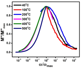
Figure 2. Scaling plot of and M” vs Frequency.

Figure 2 shows the normalized imaginary part of the electric modulus,

M^{''} / M_{\max}^{}

, plotted versus the reduced frequency

ω / ω_{\max}

for temperatures between 40°C and 500°C of NFTO ceramic. The normalization collapses the peaks onto a near-single master curve on the low-frequency side, but the overall line shape is clearly asymmetric: the high-frequency flank decays more slowly than the low-frequency flank. We tested this line shape against the standard empirical relaxation models to identify the most appropriate description.

A pure Debye relaxation (single relaxation time) predicts a perfectly symmetric master curve for

M^{''} / M_{\max}^{}

ω / ω_{\max}

. The pronounced asymmetry and the broad tails observed here therefore rule out a Debye process

[23]

. Likewise, the Cole–Cole (CC) model, which produces symmetric broadening about the peak and is parameterized by a single width parameter

α

, cannot reproduce the systematic high-frequency skew evident in the scaled data: although CC can account for the broadening visible on both flanks, it fails to capture the slower decay on the high-frequency side

[24]

The Cole–Davidson (CD) model introduces asymmetry (a stretched high-frequency tail) and qualitatively improves the fit to the observed skew. However, CD typically models a one-sided (high-frequency) stretch while keeping the low-frequency flank relatively sharp

[25]

. In the present data, the low-frequency collapse and the degree of symmetric broadening on the left flank, together with the asymmetric right flank, indicate that neither CC nor CD individually captures the full complexity of the line shape across temperatures

[18, 25]

The experimental scaling is most naturally and fully described by the Havriliak–Negami (HN) formalism, which contains two independent shape parameters (commonly labeled

α

and

γ

) and thus permits simultaneous symmetric broadening and asymmetric stretching

[26]

. The observed near-collapse on the low-frequency side implies the relaxation mechanism is the same at all temperatures (temperature chiefly shifts the characteristic time scale), while the imperfect collapse and the extended high-frequency tail imply an asymmetric distribution of relaxation times whose skewness is temperature dependent

[27]

. The HN model therefore provides the necessary flexibility to reproduce both the master-curve behavior and the asymmetric high-frequency decay visible in Figure 2.

On the basis of these observations, we adopt the Havriliak–Negami form for quantitative analysis. Practically, we perform simultaneous complex fitting of

M^{*} (ω)

(real and imaginary parts) to the HN modulus expression to extract

τ (T)

α (T)

and

γ (T)

; this approach ensures Kramers–Kronig consistency and minimizes parameter correlation. The temperature dependence of

τ

will be used to construct an Arrhenius plot and extract an activation energy for the relaxation, while the trends in

α

and

γ

will quantify how the breadth and asymmetry of the relaxation-time distribution evolve with temperature. The combined scaling and shape analysis presented here thus demonstrates a single dominant, thermally activated relaxation mechanism best described by an asymmetric, distributed HN spectrum rather than by single-time (Debye), purely symmetric (Cole–Cole) or single-sided asymmetric (Cole–Davidson) models.

5. Conclusions

A logical and logically organized discussion of the dielectric relaxation and electrical modulus formalisms has been given in this work as one spans the divide between theory and data analysis in practice. Commencing with the time-domain Debye relaxation equation, the frequency-domain expressions of complex dielectric permittivity were obtained and the physical meaning of the real and complex parts, the loss peaks as well as the geometrical representation of Cole-Cole were explained. The shortcomings of the ideal Debye model in the explanation of real materials were underlined and it inspired the emergence of empirical generalizations like the Cole-Cole, Cole-Davidson and Havriliak-Negami models to explain distributed and asymmetric relaxation times. Electrical modulus formalism was demonstrated to represent a very potent complementary representation especially where the polarization of electrodes and the conductivity of dc of the solids confound the intrinsic dielectric relaxation of the representative permittivity spectra. Debye and non-Debye models explicit relations between permittivity and modulus responses were derived which showed how modulus analysis not only moves the relaxation peaks to higher frequencies but also removes extrinsic low-frequency effects.

The use of such concepts on Nd₂FeTiO₆ ceramic showed strongly non-Debye relaxation behaviour. The asymmetric modulus arcs are depressed and scaled, and the asymmetric scaling of normalized M'' spectra of the master-curve excludes the Debye and the simple Cole-Cole description. Although the Cole-Davidson model partially explains the asymmetry, it has been found that only the Havriliak-Negami formalism can accurately reproduce the entire experimental response at all temperatures, and indicates that there is a thermally activated relaxation process where a broad and asymmetric distribution of relaxation times exists.

On the whole, it has been shown that a complex permittivity-modulus model of dielectric relaxation in disordered and conductive solids can be consistently and physically described using a combined permittivity-modulus methodology, which is examined in the context of the Havriliak-Negami model. The coherent presentation and elaborate derivations provided here are likely to benefit the students in forming conceptual knowledge and can assist the researchers in deriving meaningful relaxation parameters under the complicated dielectric and impedance spectroscopy measurements.

Abbreviations

CC	Cole-Cole
CD	Cole-Davidson
HN	Havriliak-Negami
NFTO	Nd₂FeTiO₆

Author Contributions

Mrityunjay Kumar: Conceptualization, Data curation, Methodology, Writing – original draft, Writing – review & editing

Conflicts of Interest

The author declares no conflicts of interest.

References

[1]	Schiffrin, A., Paasch-Colberg, T., Karpowicz, N., Apalkov, V., Gerster, D., Mühlbrandt, S.,... & Krausz, F. (2013). Optical-field-induced current in dielectrics. Nature, 493(7430), 70-74. https://doi.org/10.1038/nature11567
[2]	Maker, P. D., & Terhune, R. W. (1965). Study of optical effects due to an induced polarization third order in the electric field strength. Physical Review, 137(3A), A801. https://doi.org/10.1103/PhysRev.137.A801
[3]	Kirkwood, J. G. (1936). On the theory of dielectric polarization. The Journal of Chemical Physics, 4(9), 592-601. https://doi.org/10.1063/1.1749911
[4]	Buckingham, A. D. (1956). A theory of the dielectric polarization of polar substances. Proceedings of the royal society of london. series a. mathematical and physical sciences, 238(1213), 235-244. https://doi.org/10.1098/rspa.1956.0216
[5]	Choudhary, R. N. P., & Patri, S. K. (2009). Dielectric materials: introduction, research and applications (p. 152). xx: Nova Science Publishers.
[6]	Coffey, W. T. (2004). Dielectric relaxation: an overview. Journal of molecular liquids, 114(1-3), 5-25. https://doi.org/10.1016/j.molliq.2004.02.002
[7]	Nee, T. W., & Zwanzig, R. (1970). Theory of dielectric relaxation in polar liquids. The Journal of Chemical Physics, 52(12), 6353-6363. https://doi.org/10.1063/1.1672951
[8]	Drakopoulos, S. X. (2025). Revisiting the Dielectric Spectrum: Tricks and Treats of Analysis and Interpretation Around the Conductivity Relaxation. IET Nanodielectrics, 8(1), e70020. https://doi.org/10.1049/nde2.70020
[9]	Drakopoulos, S. X., Wu, J., Maguire, S. M., Srinivasan, S., Randazzo, K., Davidson, E. C., & Priestley, R. D. (2024). Polymer nanocomposites: Interfacial properties and capacitive energy storage. Progress in Polymer Science, 156, 101870. https://doi.org/10.1016/j.progpolymsci.2024.101870
[10]	Romanini, M. (2015). Relaxation dynamics in disordered systems (Doctoral dissertation, Universitat Politècnica de Catalunya).
[11]	Iglesias, T. P., Vilão, G., & Reis, J. C. R. (2017). An approach to the interpretation of Cole–Davidson and Cole–Cole dielectric functions. Journal of Applied Physics, 122(7). https://doi.org/10.1063/1.4985839
[12]	Nioua, Y., Melo, B. M. G., Prezas, P., Graça, M. F., Achour, M. E., & Costa, L. C. (2021). Analysis of the dielectric relaxation in reduced graphene oxide/epoxy composites materials using the modulus formalism. The European Physical Journal E, 44(9), 109. https://doi.org/10.1140/epje/s10189-021-00109-7
[13]	Moznine, R. E., Blanc, F., Lieutier, M., & Lefort, A. (1998). Relaxation phenomenon in composite materials. The European Physical Journal-Applied Physics, 3(2), 127-134. https://doi.org/10.1051/epjap:1998212
[14]	Blythe, A. R., & Bloor, D. (2005). Electrical properties of polymers. Cambridge university press.
[15]	Debye, P. (1934). Part I. Dielectric constant. Energy absorption in dielectrics with polar molecules. Transactions of the Faraday Society, 30, 679-684. https://doi.org/10.1039/TF9343000679
[16]	Bartnikas, R. (1983). Dielectric loss in solids. Electrical Properties of Solid Insulating Materials, (783), 3.
[17]	Cole, K. S., & Cole, R. H. (1941). Dispersion and absorption in dielectrics I. Alternating current characteristics. The Journal of chemical physics, 9(4), 341-351. https://doi.org/10.1063/1.1750906
[18]	Davidson, D. W., & Cole, R. H. (1950). Dielectric relaxation in glycerine. The Journal of Chemical Physics, 18(10), 1417-1417. https://doi.org/10.1063/1.1747496
[19]	Havriliak, S., & Negami, S. (1967). A complex plane representation of dielectric and mechanical relaxation processes in some polymers. Polymer, 8, 161-210. https://doi.org/10.1016/0032-3861(67)90021-3
[20]	Yager, W. A. (1936). The distribution of relaxation times in typical dielectrics. Physics, 7(12), 434-450. https://doi.org/10.1063/1.1745355
[21]	Halder, P., & Bhattacharya, S. (2023). Debye to non-debye type relaxation in MoO3 doped glassy semiconductors: a portrait on microstructure and electrical transport properties. Physica B: Condensed Matter, 648, 414374. https://doi.org/10.1016/j.physb.2022.414374
[22]	Macnae, J. (2025). A physical interpretation of Cole–Cole equations and their ambiguous time constants for induced polarization models. Geophysical Journal International, 243(2), ggaf362. https://doi.org/10.1093/gji/ggaf362
[23]	Elton, D. C. (2017). The origin of the Debye relaxation in liquid water and fitting the high frequency excess response. Physical Chemistry Chemical Physics, 19(28), 18739-18749. https://doi.org/10.1039/C7CP02884A
[24]	Weigand, M., & Kemna, A. (2016). Relationship between Cole–Cole model parameters and spectral decomposition parameters derived from SIP data. Geophysical Journal International, 205(3), 1414-1419. https://doi.org/10.1093/gji/ggw099
[25]	Calderwood, J. H. (2004). A physical hypothesis for Cole-Davidson behavior. IEEE transactions on dielectrics and electrical insulation, 10(6), 1006-1011. https://doi.org/10.1109/TDEI.2003.1255778
[26]	Górska, K., Horzela, A., Bratek, Ł., Dattoli, G., & Penson, K. A. (2018). The Havriliak–Negami relaxation and its relatives: the response, relaxation and probability density functions. Journal of Physics A: Mathematical and Theoretical, 51(13), 135202. https://doi.org/10.1088/1751-8121/aaafc0
[27]	Medina, J. S., Prosmiti, R., & Alemán, J. V. (2015). The role of the Havriliak-Negami relaxation in the description of local structure of Kohlrausch's function in the frequency domain. Part I. arXiv preprint arXiv: 1509.07893. https://doi.org/10.48550/arXiv.1509.07893

Cite This Article

Plain Text BibTeX RIS

APA Style

Kumar, M. (2026). Dielectric Relaxation and Electrical Modulus Formalism in Solids. Engineering Physics, 9(1), 1-9. https://doi.org/10.11648/j.ep.20260901.11

Copy | Download

ACS Style

Kumar, M. Dielectric Relaxation and Electrical Modulus Formalism in Solids. Eng. Phys. 2026, 9(1), 1-9. doi: 10.11648/j.ep.20260901.11

Copy | Download

AMA Style

Kumar M. Dielectric Relaxation and Electrical Modulus Formalism in Solids. Eng Phys. 2026;9(1):1-9. doi: 10.11648/j.ep.20260901.11

Copy | Download

@article{10.11648/j.ep.20260901.11,
  author = {Mrityunjay Kumar},
  title = {Dielectric Relaxation and Electrical Modulus Formalism in Solids},
  journal = {Engineering Physics},
  volume = {9},
  number = {1},
  pages = {1-9},
  doi = {10.11648/j.ep.20260901.11},
  url = {https://doi.org/10.11648/j.ep.20260901.11},
  eprint = {https://article.sciencepublishinggroup.com/pdf/10.11648.j.ep.20260901.11},
  abstract = {The dielectric relaxation effects give a very important understanding of the microscopic dynamics of dipoles and charge carriers in solids, especially those materials where disorder, conductivity and interfacial effects make the dielectric response difficult to understand. A single and pedagogic exposition of dielectric relaxation in this work is introduced, starting with the analogous time domain Debye polarization equation and moving stepwise to the frequency domain complex permittivity formulation. Real and complex values of the dielectric permittivity are obtained and their physical interpretation, loss peak performance and Cole Cole presentation are provided in details. Abnormal Debye behaviour in real solids is treated by the Cole-Cole, Cole-Davidson and Havriliak-Negami models, which are focused on the characteristics of describing distributed and asymmetric relaxation-time spectra. In order to by-pass the restrictions due to the conductivity of the dc and as polarization of the electrodes at low frequencies, electrical modulus formalism is presented and derived in the case of Debye and non-Debye relaxation model. The usefulness of this method is illustrated by the fact that the complex modulus spectra of Nd2FeTiO6 ceramic were analyzed in the entire span of temperatures. The presence of depressed and asymmetric modulus arcs, scaled master-curve behavior also obviously signal non-Debye relaxation behavior best fitted by the HavriliakNegami model. The joint analysis of permittivity-modulus offers a powerful model of isolating the intrinsic bulk relaxation and extrinsic conductive sources, and can be used to obtain physically useful relaxation parameters. The work is not only an introduction on a tutorial level, but also a practical guide to researchers working on dielectric and impedance spectroscopy of solid materials.},
 year = {2026}
}

Copy | Download

TY  - JOUR
T1  - Dielectric Relaxation and Electrical Modulus Formalism in Solids
AU  - Mrityunjay Kumar
Y1  - 2026/05/13
PY  - 2026
N1  - https://doi.org/10.11648/j.ep.20260901.11
DO  - 10.11648/j.ep.20260901.11
T2  - Engineering Physics
JF  - Engineering Physics
JO  - Engineering Physics
SP  - 1
EP  - 9
PB  - Science Publishing Group
SN  - 2640-1029
UR  - https://doi.org/10.11648/j.ep.20260901.11
AB  - The dielectric relaxation effects give a very important understanding of the microscopic dynamics of dipoles and charge carriers in solids, especially those materials where disorder, conductivity and interfacial effects make the dielectric response difficult to understand. A single and pedagogic exposition of dielectric relaxation in this work is introduced, starting with the analogous time domain Debye polarization equation and moving stepwise to the frequency domain complex permittivity formulation. Real and complex values of the dielectric permittivity are obtained and their physical interpretation, loss peak performance and Cole Cole presentation are provided in details. Abnormal Debye behaviour in real solids is treated by the Cole-Cole, Cole-Davidson and Havriliak-Negami models, which are focused on the characteristics of describing distributed and asymmetric relaxation-time spectra. In order to by-pass the restrictions due to the conductivity of the dc and as polarization of the electrodes at low frequencies, electrical modulus formalism is presented and derived in the case of Debye and non-Debye relaxation model. The usefulness of this method is illustrated by the fact that the complex modulus spectra of Nd2FeTiO6 ceramic were analyzed in the entire span of temperatures. The presence of depressed and asymmetric modulus arcs, scaled master-curve behavior also obviously signal non-Debye relaxation behavior best fitted by the HavriliakNegami model. The joint analysis of permittivity-modulus offers a powerful model of isolating the intrinsic bulk relaxation and extrinsic conductive sources, and can be used to obtain physically useful relaxation parameters. The work is not only an introduction on a tutorial level, but also a practical guide to researchers working on dielectric and impedance spectroscopy of solid materials.
VL  - 9
IS  - 1
ER  -

Copy | Download

Author Information

Mrityunjay Kumar

Department of Physics, Shaheed Harchand Naik Govt. College, Tokapal, India; University Department of Physics, Ranchi University, Ranchi, India

Contact Email

http://orcid.org/0009-0000-0709-8117

Download PDF

Submit an Article

Plain Text BibTeX RIS

APA Style

Kumar, M. (2026). Dielectric Relaxation and Electrical Modulus Formalism in Solids. Engineering Physics, 9(1), 1-9. https://doi.org/10.11648/j.ep.20260901.11

Copy | Download

ACS Style

Kumar, M. Dielectric Relaxation and Electrical Modulus Formalism in Solids. Eng. Phys. 2026, 9(1), 1-9. doi: 10.11648/j.ep.20260901.11

Copy | Download

AMA Style

Kumar M. Dielectric Relaxation and Electrical Modulus Formalism in Solids. Eng Phys. 2026;9(1):1-9. doi: 10.11648/j.ep.20260901.11

Copy | Download

@article{10.11648/j.ep.20260901.11,
  author = {Mrityunjay Kumar},
  title = {Dielectric Relaxation and Electrical Modulus Formalism in Solids},
  journal = {Engineering Physics},
  volume = {9},
  number = {1},
  pages = {1-9},
  doi = {10.11648/j.ep.20260901.11},
  url = {https://doi.org/10.11648/j.ep.20260901.11},
  eprint = {https://article.sciencepublishinggroup.com/pdf/10.11648.j.ep.20260901.11},
  abstract = {The dielectric relaxation effects give a very important understanding of the microscopic dynamics of dipoles and charge carriers in solids, especially those materials where disorder, conductivity and interfacial effects make the dielectric response difficult to understand. A single and pedagogic exposition of dielectric relaxation in this work is introduced, starting with the analogous time domain Debye polarization equation and moving stepwise to the frequency domain complex permittivity formulation. Real and complex values of the dielectric permittivity are obtained and their physical interpretation, loss peak performance and Cole Cole presentation are provided in details. Abnormal Debye behaviour in real solids is treated by the Cole-Cole, Cole-Davidson and Havriliak-Negami models, which are focused on the characteristics of describing distributed and asymmetric relaxation-time spectra. In order to by-pass the restrictions due to the conductivity of the dc and as polarization of the electrodes at low frequencies, electrical modulus formalism is presented and derived in the case of Debye and non-Debye relaxation model. The usefulness of this method is illustrated by the fact that the complex modulus spectra of Nd2FeTiO6 ceramic were analyzed in the entire span of temperatures. The presence of depressed and asymmetric modulus arcs, scaled master-curve behavior also obviously signal non-Debye relaxation behavior best fitted by the HavriliakNegami model. The joint analysis of permittivity-modulus offers a powerful model of isolating the intrinsic bulk relaxation and extrinsic conductive sources, and can be used to obtain physically useful relaxation parameters. The work is not only an introduction on a tutorial level, but also a practical guide to researchers working on dielectric and impedance spectroscopy of solid materials.},
 year = {2026}
}

Copy | Download

TY  - JOUR
T1  - Dielectric Relaxation and Electrical Modulus Formalism in Solids
AU  - Mrityunjay Kumar
Y1  - 2026/05/13
PY  - 2026
N1  - https://doi.org/10.11648/j.ep.20260901.11
DO  - 10.11648/j.ep.20260901.11
T2  - Engineering Physics
JF  - Engineering Physics
JO  - Engineering Physics
SP  - 1
EP  - 9
PB  - Science Publishing Group
SN  - 2640-1029
UR  - https://doi.org/10.11648/j.ep.20260901.11
AB  - The dielectric relaxation effects give a very important understanding of the microscopic dynamics of dipoles and charge carriers in solids, especially those materials where disorder, conductivity and interfacial effects make the dielectric response difficult to understand. A single and pedagogic exposition of dielectric relaxation in this work is introduced, starting with the analogous time domain Debye polarization equation and moving stepwise to the frequency domain complex permittivity formulation. Real and complex values of the dielectric permittivity are obtained and their physical interpretation, loss peak performance and Cole Cole presentation are provided in details. Abnormal Debye behaviour in real solids is treated by the Cole-Cole, Cole-Davidson and Havriliak-Negami models, which are focused on the characteristics of describing distributed and asymmetric relaxation-time spectra. In order to by-pass the restrictions due to the conductivity of the dc and as polarization of the electrodes at low frequencies, electrical modulus formalism is presented and derived in the case of Debye and non-Debye relaxation model. The usefulness of this method is illustrated by the fact that the complex modulus spectra of Nd2FeTiO6 ceramic were analyzed in the entire span of temperatures. The presence of depressed and asymmetric modulus arcs, scaled master-curve behavior also obviously signal non-Debye relaxation behavior best fitted by the HavriliakNegami model. The joint analysis of permittivity-modulus offers a powerful model of isolating the intrinsic bulk relaxation and extrinsic conductive sources, and can be used to obtain physically useful relaxation parameters. The work is not only an introduction on a tutorial level, but also a practical guide to researchers working on dielectric and impedance spectroscopy of solid materials.
VL  - 9
IS  - 1
ER  -

Copy | Download