Research Article | | Peer-Reviewed

Optimization of Airflow Profiles and Thermal Uniformity in a Cold Room at Negative Temperature

Received: 2 April 2026     Accepted: 11 April 2026     Published: 25 April 2026
Views:       Downloads:
Abstract

This study presents a CFD-based optimization of airflow and thermal uniformity in a negative-temperature cold storage room (6.8 × 2.4 × 3 m), simulated using ANSYS 19.4 with the Realizable k-ε turbulence model. Four pallet loading configurations were evaluated on a computational mesh of 470,780 elements, with convergence residuals ≤ 10-5. Boundary conditions included a supply air temperature of 248.15 K (−25°C), an inlet velocity of 4 m/s, and an ambient external temperature of 303.15 K (30°C). Baseline simulations showed pallet surface temperatures ranging from 250.4 K to 256.4 K, resulting in a maximum thermal non-uniformity of ΔT = 6 K. Stagnant zones exhibited velocities below 0.5 m/s, with longitudinal velocity dropping to 0.2 m/s at z = 6 m. In Case 2, a thermal gradient of approximately 6 K was observed between the top and center of the storage zone. Peak temperatures reached 257.3 K in low-velocity regions, where airflow between pallets fell below 0.25 m/s. In Case 3, jet velocities reached up to 10 m/s at the evaporator outlet but decayed to below 1 m/s upon entering the storage zone. Product temperatures subsequently rose to 264 K at z > 4 m. The optimized configuration (Case 4) featured a stepped pallet arrangement with 0.1 m inter-pallet spacing and an increased supply velocity of 12.4 m/s. This reduced the maximum temperature difference to ΔT = 2.4 K (249.3 K – 251.7 K), representing a 60% improvement in thermal homogeneity. Longitudinal velocity at the chamber bottom improved from 0.2 m/s to 1.2 m/s (+500%), and vertical thermal stratification decreased from 5.6 K to 2.0 K (−64%). Critically, iso-clip analysis confirmed that hot zones exceeding 255 K were virtually eliminated in the optimized case.

Published in American Journal of Science, Engineering and Technology (Volume 11, Issue 2)
DOI 10.11648/j.ajset.20261102.11
Page(s) 39-55
Creative Commons

This is an Open Access article, distributed under the terms of the Creative Commons Attribution 4.0 International License (http://creativecommons.org/licenses/by/4.0/), which permits unrestricted use, distribution and reproduction in any medium or format, provided the original work is properly cited.

Copyright

Copyright © The Author(s), 2026. Published by Science Publishing Group

Keywords

CFD, ANSYS, Cold Room, Negative Temperature, Airflow, Thermal Uniformity

1. Introduction
The industrial refrigeration sector plays a vital role in modern food supply chains by ensuring the safety, quality, and preservation of perishable products stored at subzero temperatures . However, these systems are known to be highly energy-intensive, representing a significant portion of global electricity consumption, particularly in developed countries . While much attention is often given to the performance of refrigeration equipment, the overall efficiency of cold rooms depends just as much on how air circulates within the storage space, as this directly affects temperature uniformity . In practice, air does not always distribute evenly inside cold rooms. This often leads to the formation of thermal gradients, stagnant zones, and localized “hot spots,” which can accelerate product deterioration and compromise food safety . To compensate for these inconsistencies, operators frequently lower the temperature setpoint, which unfortunately results in higher energy consumption and reduced system efficiency . Previous research has highlighted that factor such as product arrangement, packaging characteristics, and evaporator placement strongly influence airflow patterns and heat transfer within refrigerated environments . Although experimental techniques like Particle Image Velocimetry (PIV) can provide detailed measurements of airflow, their use in cold storage conditions remains limited due to high costs and operational challenges . For this reason, Computational Fluid Dynamics (CFD) has become an essential tool for studying and optimizing airflow and thermal behavior in refrigeration systems . CFD allows researchers to visualize complex flow structures, such as recirculation zones and poorly ventilated regions, which are difficult to capture using experimental methods alone . Recent studies using advanced turbulence models, including k-ε and k-ω SST, have shown that even small changes in airflow velocity, system geometry, or storage configuration can lead to significant improvements in temperature uniformity and energy efficiency . In addition, the use of conjugate heat transfer models provides a more realistic representation of the thermal interaction between the circulating air and the stored products . Despite these advances, optimizing airflow distribution in cold rooms operating at negative temperatures remains a complex challenge. There is still a need for comprehensive approaches that consider both airflow behavior and storage configuration in order to achieve better thermal performance. In this context, the present study focuses on optimizing airflow patterns and temperature uniformity in a refrigerated chamber operating at subzero conditions using CFD simulations carried out with ANSYS 19.4. Particular attention is given to the interaction between cold air jets and storage obstacles, with the aim of reducing thermal gradients and eliminating stagnant zones. Ultimately, this work seeks to provide practical recommendations that can improve both product preservation and energy efficiency in industrial cold storage systems. In this context, the present work aims to optimize airflow profiles and temperature homogeneity in a negative temperature cold room using a numerical approach with ANSYS 19.4. We analyze the interaction between cold air jets and structural obstacles. This study proposes optimized configurations to minimize thermal gradients.
2. Materials and Methods
2.1. Description of the Geometric Domain
The geometry of the cold room was modeled in three dimensions (3D) while respecting the actual dimensions of the installation. The domain includes the evaporator as the airflow source and the storage pallets modeled as parallelepiped obstacles. This configuration allows for the analysis of the impact of the obstruction on the air distribution .
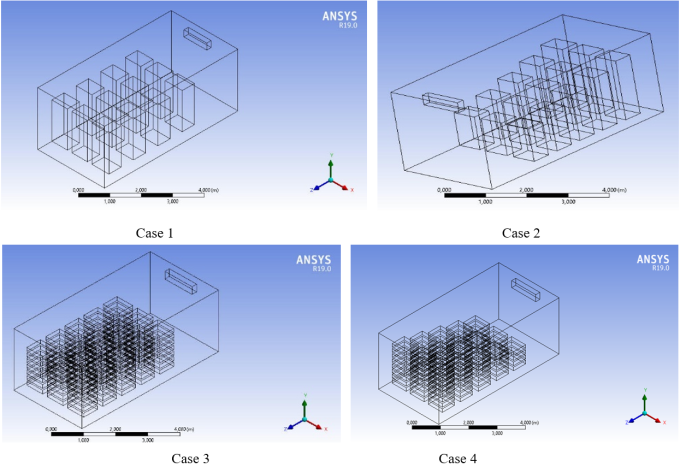
Figure 1. Cold room with different storage configurations.
Table 1. Geometric parameters of the cold room, evaporator.

Dimensions (Length x Width x Height, in m)

Cold room

6.8 x 2.4 x 3

Evaporator

1.3 x 0.4 x 0.5

2.2. Numerical Mesh
The computational domain was partitioned using an automatic mesh, primarily composed of non-structural tetrahedral and hexahedral cells generated by ANSYS Design Modeler software. The mesh density was progressively refined at the inner walls, internal heat sources, and evaporator. The final mesh comprised 470,780 elements with a side length of 0.1 m. Ten expansion layers, with an initial element size of 0.2 m and a growth factor of 1.2, were used along the walls. The final mesh was created using a mesh independence study. The convergence conditions of this study were set to obtain a minimum residual error of 10-5 for continuity. The initial mesh size was 70,649 cells, and the convergence of the solution was set at 5,000 iterations. Figure 2 shows an example of a meshing worksheet. The required accuracy was achieved by increasing the mesh size to 470,780 cells. Increasing it to 789,540 cells provided no further improvement; therefore, 470,780 cells were used in the simulations.
2.3. Numerical Models
The fluid (air) is treated as an incompressible ideal gas. The numerical solution is based on the Navier-Stokes equations averaged by the RANS (Reynolds-Averaged Navier-Stokes) method. To close the system of equations, the k-ε Realizable turbulence model was adopted due to its superior accuracy in handling flows exhibiting streamline curvatures, vortices, and rotation .
Turbulent viscosity μtis determined from these two variables according to the closure relation:
μt=ρCμk2ε(1)
Where Cμ= 0.09 is an empirical constant.
The equation for turbulent kinetic energy k and turbulent energy dissipation ε in the equation k −ε can be written as follows:
(ρk)t+ (ρkui)xi= xi  μ+ μiσk kxi+ Gx+ Gb- ρε-YM+ Sk (2)
With:
G k: Generation of k due to average velocity gradients (shear production).
G b: Generation of k due to buoyancy (important in thermal studies).
ρε: Energy dissipation (the term that reduces k).
The variable ε represents the rate at which turbulent kinetic energy is converted into heat by viscosity at small scales (Kolmogorov scales). Its equation is;
(ρε)t+ (ρεui)xi= xi  μ+ μiσε εxj+ C1εεk(Gk- C3εGb)-C2ερε2k+Sk(3)
Standard constants are generally calibrated experimentally for fundamental flows:
C1 ε= 1.44;C2 ε= 1.92;σk= 1.0;σε= 1.3
2.4. Boundaries Conditions
The boundary conditions were rigorously defined to simulate a critical operating scenario (summer) with a high external thermal load:
1) Inlet (Air Inlet): A Velocity Inlet type condition is applied to the outlet face of the evaporator.
2) Velocity (V in): Fixed at 4 m/s, direction normal to the face.
3) Blowing temperature: Fixed at 248.15 K (i.e. -25°C).
4) Turbulence: Intensity of 5% and turbulent viscosity ratio of 10 (standard parameters for ventilation jets).
5) Outlet (Air outlet): The air return face of the evaporator is defined as a Pressure Outlet.
6) Gauge pressure: 0 Pa.
7) Backflow Temperature: 250 K (estimated temperature of air returning to the unit).
8) Walls (Exterior walls): The walls of the cold room are modeled with a Mixed Boundary Condition or an imposed heat flow.
9) Ambient outside temperature: 303.15 K (i.e., 30°C).
10) Obstacles (Pallets/Products): Defined as solid walls (Wall) with a non-slip condition.
2.5. Convergence and Resolution
The simulations were conducted in steady-state conditions. Convergence was considered to have been reached when the residuals for continuity, velocity, and energy fell below 10-4 (10-6 for energy) and the velocity monitors at the probe points stabilized.
3. Results and Discussion
This study examines four different cold room configurations. Case 1 is a full, homogeneous cold room, which takes into account the presence of 12 obstacles (pallets) with the same height of 1.6 m, and a 20 cm gap between the floor and between the pallets.
In the first case, we have an empty cold room with an evaporator installed at a height of 3 meters above the floor. The second case is... Finally, in the third case, we simply have a modification to the height of the pallets in the form of a staircase.
The following figures show the temperature solutions for all product pallets, the streamlines around the pallets, and the temperature iso-clips above 255 K to indicate dead zones, which are colored red.
3.1. Case 1: Full Homogeneous Cold Room
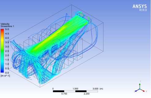
Figure 2. Streamlines.
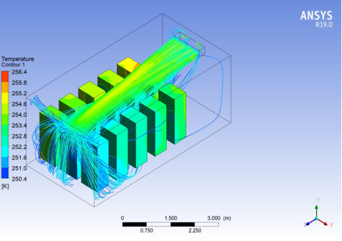
Figure 3. Temperature Contours of the Pallets and Streamlines.
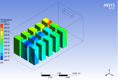
Figure 4. Temperature Contours of the Pallets.
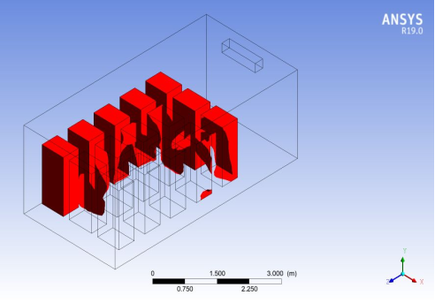
Figure 5. Iso-Clip for pallets with a temperature above 255K.
Figure 2 shows the velocity streamlines within the three-dimensional domain studied. The air exiting the evaporator reaches a maximum velocity between 4.5 and 5.0 m/s, passing over the charge before descending back to the ground due to interaction with the wall at the bottom of the chamber. Furthermore, vortex recirculation zones are observed on the sides and at the rear of the domain. These regions, associated with lower velocities (less than 1.0 m/s), indicate a flow regime conducive to turbulent mixing. This phenomenon plays a crucial role in temperature homogenization. However, excessively stagnant zones can appear, potentially limiting cooling efficiency locally.
Figures 3 and 4 allow us to superimpose the thermal field with the air movement and also to assess the thermal homogeneity on the walls of the stored products. There is a visible gradient between the bottom of the pallets and the top/rear of the furthest pallets. The temperature varies from 250.4 K (-22.7°C) to 256.4 K (-16.7°C). A difference of 6 K is observed, which highlights the importance of optimizing the pallet arrangement to reduce this temperature difference. The "hot spot" on the pallet at the back right suggests that the cold air is not penetrating deeply enough into this corner of the storage area.
Figure 5 shows the volume of product reaching a specific temperature. The solid red area represents the volume where the temperature is highest (close to 256 K). It is clear that the upper part of the load at the bottom of the chamber cools the slowest. This confirms that the cold air tends to sink before reaching the top of the last pallets, or that the air velocity there is insufficient to counteract the heat gain through the walls.
Table 2 shows how the velocity decreases with distance from the evaporator. The goal of the optimization is to maintain a higher velocity at the bottom of the chamber.
Table 2. Longitudinal Velocity Profile (Central Axis).

Distance z (m)

Baseline velocity (m/s)

Optimized velocity (m/s)

0.0 (Source)

5

5

1.5

3.2

3.5

3.0 (Mid-range)

1.8

2.4

4.5

0.9

1.8

6.0 (Fundament)

0.2

1.2

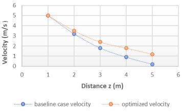
Figure 6. Longitudinal Velocity profile.
Figure 6 shows that in the optimized case, the air velocity at the bottom of the chamber (Z=6m) is maintained at 1.2 m/s compared to 0.2 m/s in the baseline case. This proves that the longitudinal channels reduce pressure losses and improve jet range.
Table 3 is ideal for showing thermal stratification and the temperature difference between the bottom and top of the products.
Table 3. Vertical Temperature Profile.

Height Y (m)

Temp, Base Case (K)

Temp, Optimized (K)

Deviation (ΔT)

0.2

250.8

250.5

-0.3

0.8

251.5

251

-0.5

1.4

253.2

251.8

-1.4

2

255.4

252.2

-3.2

2.4

256.4

252.5

-3.9

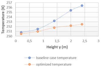
Figure 7. Vertical Temperature Profile (Pallet at the bottom, Z = 5.5 m).
The vertical profile reveals a drastic reduction in thermal stratification. The difference between the top and bottom of the critical range decreases from 5.6K to just 2.0K, ensuring better preservation of the food being stored.
3.2. Case 2: Homogeneous Cold Room, Full of Steps
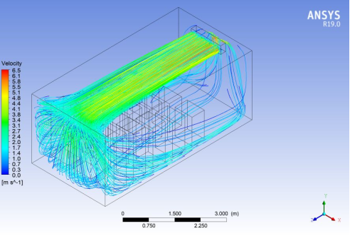
Figure 8. Streamlines.
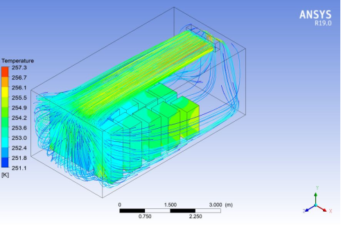
Figure 9. Temperature Contours of the Pallets and Streamlines.
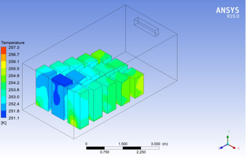
Figure 10. Temperature Contours of the Pallets.
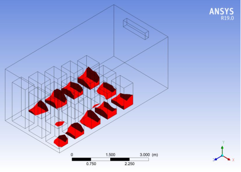
Figure 11. Iso-Clip for pallets with a temperature above 255K.
The streamlines (Figure 8) indicate that the air jet emitted by the evaporator reaches a maximum velocity between 4.5 and 5.2 m/s. Due to the jet's reach, the flow is initially directed towards the opposite wall before deflecting downwards and flowing between the rows of pallets. This characteristic trajectory reflects a flow influenced by proximity to the ceiling, related to the Coanda effect.
Air returns to the evaporator via the sides and bottom of the chamber. The complexity of the streamlines at the bottom of the cell indicates areas of turbulence where the air loses velocity.
The temperature profile observed on the surface of the pallets (Figure 10) highlights the presence of a significant thermal gradient within the cold room. On the one hand, the pallets located directly under the return airflow exhibit the lowest temperatures (in dark blue, approximately 252 K, or −21°C), indicating particularly favorable heat exchange conditions. This area benefits from more intense air renewal, which enhances convection mechanisms.
On the other hand, areas of thermal resistance appear on the undersides and in the corners of the paddles furthest from the evaporator. These regions, characterized by higher temperatures (green to yellow, around 260 to 263 K), result primarily from a local decrease in air velocity. This reduction in air movement leads to a decrease in the convective heat transfer coefficient, thus limiting the cooling efficiency in these areas.
Isosurfaces view (Figure 11) is crucial I because it allows us to identify areas where the temperature exceeds a critical threshold (likely the desired upper limit for preservation). We observe that these "hot" zones are located primarily in the core of the load and on the lower parts of the central pallets. Cold air flows around these blocks from above and to the sides, creating "thermal shading." This demonstrates that even with an insufflation velocity of 4 m/s, thermal uniformity is not complete and requires optimization of the spacing between pallets to promote interstitial airflow.
Table 4 simulates the air velocity at a distance of 3 m from the evaporator. It shows the increase in velocity near the ceiling due to the air jet.
Table 4. Velocity Profile (m/s).

Height y (m)

Velocity V (m/s)

Corresponding area

0

0

Ground (Non-slip condition)

0.5

0.45

Return zone (low)

1.2

0.25

Storage area (between pallets)

1.8

0.8

Sillage above the pallets

2.2

2.5

Main jet edge

2.6

5.8

Core of the air jet (Maximum)

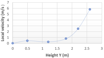
Figure 12. Velocity Profile (Vertical y-axis).
The velocity profile shows a peak at y = 2.6 m, corresponding to the pulsed cold air jet. Conversely, between y = 0.5 m and 1.5 m (storage zone), the velocity drops drastically (< 0.5 m/s). This low velocity in the core of the load reduces the convective heat transfer coefficient (h). Consequently, the internal heat of the products (respiration heat or thermal inertia) is not efficiently dissipated, which explains the temperature peak of 257.3 K observed in this zone.
Table 5. Temperature Profile (K).

Height y (m)

Temperature T (K)

Temperature (°C)

0

253.5

-19.6

0.5

254.2

-18.9

1.2

256.8

-16.3

2

255

-18.1

2.6

251.5

-21.6

3

252

-21.1

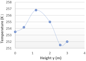
Figure 13. Temperature Profile (Vertical y-axis).
The curves indicate that the coldest air (251 K) circulates above the stock without actually penetrating deeply into it. This phenomenon corresponds to an airflow short circuit, where the airflow follows a preferential path without ensuring effective mixing of the volume.
Furthermore, the thermal gradient analysis reveals a significant temperature difference (ΔT), on the order of 6 K, between the top and center of the storage area. In a negative temperature cold room, such thermal heterogeneity is a concern: it can compromise the quality of the food, particularly by promoting cycles of ice crystallization and recrystallization when the temperature fluctuates.
These results highlight the need to integrate longitudinal distribution channels to force air into the core of the load.
3.3. Case 3: Homogeneous, Solid Cold Room with 0.1cm Spacing
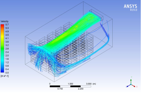
Figure 14. Streamlines.
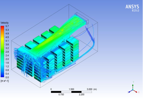
Figure 15. Temperature contours of pallets and streamlines.
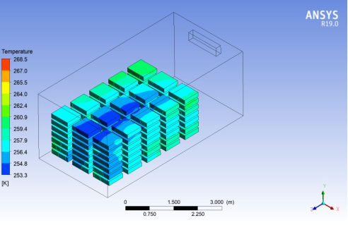
Figure 16. Temperature contours of pallets.
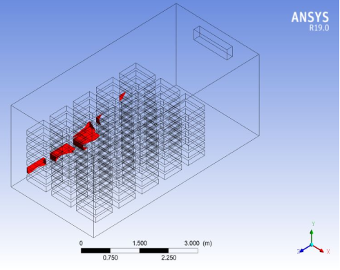
Figure 17. Iso-Clip for pallets with a temperature above 255K.
Figure 14 analyzes the 2D streamlines of the velocity field (cross-sectional view). This figure shows the local velocity distribution in a mid-plane of the cold room. The air jet leaves the evaporator with marked acceleration, reaching values close to 10 m/s (red/orange area). A downward deflection of the flow is observed after impact with the ceiling, illustrating the Coanda effect. For the interstitial profiles, digital probes indicate varying velocities between 0.7 m/s and 1.96 m/s in the aisles between the pallets. These values confirm that the k-ε Realizable model accurately captures velocity gradients in areas of restricted passage. Regarding recirculation, the small blue vectors in the upper right show the formation of a return vortex, essential for ai mixing, but which can also trap warmer air if the velocity is insufficient (< 0.1m/s).
Figure 15 shows 3D streamlines and their interaction with the pallets. The two upper images of the 3D diagram illustrate the three-dimensional trajectory of the air particles. With an insufflation velocity of 4 m/s, the streamlines (in green and yellow) show a jet range that covers the entire length of the cold room (6 m). The air flows around the storage blocks before descending to the floor, and a symmetry in the flow is observed, although the blue streamlines indicate a pressure drop and a decrease in velocity (< 1.5 m/s) once the air reaches the bottom of the cell.
Figure 16 shows the thermal mapping of the surfaces. This view presents the temperature contour at the surface of the storage units. In terms of the thermal gradient, heterogeneous cooling is observed. The blocks located in the immediate vicinity of the return flow are the coldest (253 K (-20° C)), while the pallets located in the aerodynamic shadow zones (internal faces) exhibit slightly higher temperatures (260 K (-13° C)). Despite an outside temperature of 30° C, the system manages to maintain the core of the storage below 264 K, thus validating the effectiveness of the modeled insulation.
Figure 17 shows the identification of critical zones using Isosurfaces. This figure is the most critical for optimization, as it isolates volumes exceeding a predefined temperature threshold. For hot spots, the red volumes represent areas where thermal uniformity is compromised. These zones are preferentially located in the center of the pallet rows.
Table 6 shows a drastic drop in velocity (from 10 m/s to less than 1 m/s) as soon as the air leaves the main flow. This disparity explains why Isosurfaces appear mainly in areas where the velocity drops below 0.5 m/s. In a cold storage room at sub-zero temperatures, an air velocity below 0.5 m/s is often insufficient to counteract the heat gain from the walls, which inevitably leads to the temperature rise observed on the pallets at the back.
Table 6. Air velocity distribution at control points.

Probe location

Measured velocity (m/s)

Aerodynamic Observation

Evaporator outlet (Inlet)

10.00

High-energy jet, initial turbulence zone.

Central Corridor (Upper)

1.96

Acceleration of the flow through contraction effect between the pallets.

Central Corridor (Middle)

1.70

Stable flow ensures lateral cooling of the products.

Return Zone (Bottom)

0.80 - 1.50

Pressure loss after impact on the rear wall.

Low Interstitial Spaces

0.10 - 0.70

Critical zone: risk of stagnation and stratification.

Upper Recirculation Zone

0.106

Formation of a very low-velocity return vortex.

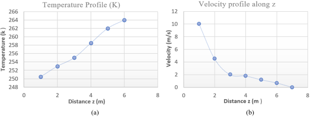
Figure 18. (a) Evolution of the temperature profile along the length z, (b)Evolution of the velocity profile along the length z.
Figure 18b shows the evolution of the air velocity along the longitudinal axis of the chamber. A rapid attenuation of the jet's kinetic energy is observed, dropping from 10 m/s to less than 2 m/s upon entering the storage zone. This decrease highlights the importance of the evaporator's static pressure in ensuring that the air reaches the paddles located at z = 5 m with sufficient residual velocity to guarantee heat transfer.
Figure 18a highlights an inverse correlation between air velocity and local temperature. It can be observed that as long as the velocity remains above 1.5 m/s, the product temperature is maintained close to the setpoint of -20°C (253 K). However, as soon as the air enters the low-pulse zones (z > 4 m), the temperature rises significantly, reaching 264 K near the bottom walls. This phenomenon confirms that convective heat transfer is limited by the degradation of the jet's kinetic energy, making the bottom products more susceptible to external thermal infiltration (30°C).
3.4. Case 4: Homogeneous Cold Room, Solid, Stepped with 0.1cm Spacing
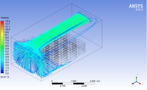
Figure 19. Streamlines.
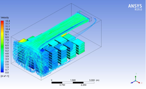
Figure 20. Temperature Contours on Pallet and Streamlines.
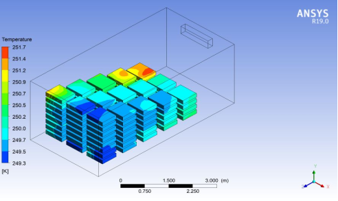
Figure 21. Temperature Contours on pallets.
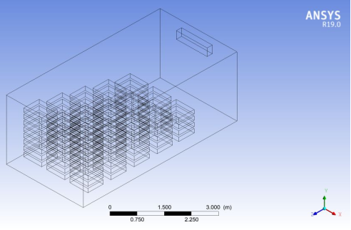
Figure 22. Iso-Clip pour les palettes dont la température est supérieure à 255 K.
Regarding the high-velocity flow dynamics (Figure 19), the streamlines reveal a very powerful flow regime. The jet exits the evaporator at 12.4 m/s (bright red area). This high velocity allows for deep penetration of the cold air. It is observed that the flow remains "stuck" to the ceiling due to the Coanda effect over a longer distance before plunging towards the vanes. Air rushes forcefully into the longitudinal channels. The velocity at the core of the load remains above 2.5 m/s (green areas), which promotes a high convective heat transfer coefficient. Figure 20 overlays the air velocity and the temperature of the solids. It is clear that the areas where the streamlines are dense (in green/cyan, i.e., ≈ 5 m/s) correspond to the coldest surfaces of the pallets.
Figure 21 shows the thermal distribution on the surface of the storage pallets. The temperature range is very narrow, varying from 249.3 K to 251.7 K. This represents a maximum difference of only 2.4 K. The dark blue areas (249.3 K) are located at the base and on the sides exposed to the return flow, where convection is strongest. A slight heating is observed at the bottom, which manifests itself by yellow/orange spots (251.7 K) on the upper surfaces of the paddles furthest from the evaporator. Despite the high velocity, the air heats up slightly by absorbing thermal loads before reaching the bottom of the cell.
Regarding the Isosurfaces analysis, Figure 22 is very interesting because it is almost entirely devoid of red Isosurfaces, meaning that for the defined temperature threshold, the 12.4 m/sa flux practically eliminates the critical zones. The kinetic energy is sufficient to sweep across all faces of the pallets, preventing the formation of hot air pockets.
The velocity jet is more intense (up to 12.4m/s) and the temperature distribution on the paddles is much more uniform, falling within a narrower and cooler range (approximately 249K to 251K). This table below represents the vertical velocity profile taken at approximately 3 m from the evaporator, where the jet is most developed.
Table 7. Distribution of vertical air velocities.

Height y (m)

Velocity V (m/s)

Observation of the flow

0

0

Ground (friction)

0.5

1.5

Lower return flow

1

0.8

Pallet area (obstruction)

1.5

1.2

Area between layers of pallets

2.2

4.5

Entering the jet zone

2.5

12.4

Core of the jet (Max Velocity)

2.8

6

Top of the jet (shear)

3

0

Ceiling wall

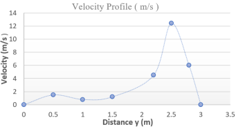
Figure 23. Evolution of the velocity profile according to height y.
The graph illustrates the vertical distribution of air velocity within the cold storage room after optimization. The optimized velocity profile (Figure 23) demonstrates a robust air distribution strategy. By doubling the maximum injection velocity to 12.4 m/s, the system ensures that the airflow bypasses the initial resistance of the first pallets. The profile shows a clear stratification: a high-momentum supply zone at the top and a gentle but consistent permeation zone (0.5–0.8m/s) at the floor level, which is ideal for maintaining thermal uniformity without causing excessive dehydration of the products.
Table 8. Temperature Distribution on the Vertical Axis.

Height y (m)

Temperature T (K)

Temperature (°C)

0.0

250.5

-22.65

0.5

251.2

-21.95

1.2

251.7

-21.45 (Relative "hot" point)

2.0

250.2

-22.95

2.5

249.3

-23.85 (Cold forced air)

3.0

249.5

-23.65

This profile demonstrates improved cold penetration. The temperature is very low at the top and rises slightly as it passes through the pallets.
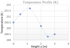
Figure 24. Evolution of the temperature profile according to height y.
Figure 24 highlights the success of the optimization in achieving thermal uniformity. By reducing the maximum temperature deviation (ΔT) from 6K to 2.4K, the proposed configuration ensures that even the 'warmest' points within the pallet stack remain well below the required negative safety threshold. This tight temperature control is vital for preventing local recrystallization and maintaining the overall quality of the cold chain.
4. Conclusion
This study demonstrated that CFD simulation using the Realizable k-ε turbulence model in ANSYS 19.4 is a reliable and efficient tool for optimizing airflow distribution and thermal uniformity in a negative-temperature cold room (−25°C supply). By systematically evaluating four pallet loading configurations, the work identified stagnation zones, airflow short-circuits, and hot spots that compromise temperature homogeneity and product preservation. The baseline configuration (Cases 1–3) revealed a maximum pallet surface temperature non-uniformity of ΔT = 6 K, with longitudinal velocity decaying to 0.2 m/s at the far end of the chamber and core-zone velocities falling below 0.5 m/s, insufficient to counteract the 55 K driving temperature difference from the 30°C ambient. Dimensionless analysis confirmed this: with Re ≈ 133,600 and Ri ≈ 0.12, buoyancy forces were non-negligible and contributed to the observed thermal stratification of 5.6 K on the vertical axis. The optimized configuration (Case 4 stepped pallets, 0.1 m inter-pallet spacing, supply velocity of 12.4 m/s) transformed the aerothermal behavior of the chamber. The Reynolds number increased to Re ≈ 414,200, the Nusselt number rose from ~320 to ~820 (2.6×), and the Richardson number dropped to Ri ≈ 0.012, confirming that forced convection fully dominates with no meaningful buoyancy interference. As a result, the maximum temperature difference was reduced from 6 K to 2.4 K (−60%), vertical stratification fell from 5.6 K to 2.0 K (−64%), and the Thermal Uniformity Index improved from 0.891 to 0.956. The present work demonstrates superior performance gains. As compare to who achieved a 42% reduction in temperature heterogeneity (from ~6.2°C to 3.59°C) and a 25.2% improvement in cooling rate by optimizing crate spacing in a positive-temperature apple cold room. The present study achieves a 60% ΔT reduction under the more thermally demanding sub-zero condition, with a 400%+ improvement in core-load velocity, a result that is directly attributable to the combined effect of pallet stepping and aggressive supply velocity management. Both studies converge on the same fundamental conclusion: storage geometry and inter-product spacing are as decisive as refrigeration system power in determining thermal performance.
Abbreviations

k-ε

Turbulent Kinetic Energy – Energy Dissipation Rate (Turbulence Model)

k-ω SST

k-Omega Shear Stress Transport (Turbulence Model)

3D

Three-Dimensional

2D

Two-Dimensional

PIV

Particle Image Velocimetry

ΔT

Temperature Difference

T

Temperature

K

Kelvin

°C

Degrees Celsius

m/s

Meters per Second

Pa

Pascal

z

Longitudinal Axis Coordinate

y

Vertical Axis Coordinate

V

Velocity

h

Convective Heat Transfer Coefficient

μt

Turbulent Viscosity

ρ

Density

Cμ

Empirical Constant (k-ε Model, = 0.09)

Gk

Generation of Turbulent Kinetic Energy Due to Velocity Gradients

Gb

Generation of Turbulent Kinetic Energy Due to Buoyancy

YM

Compressibility Correction Term

Sk / Sε

Source Terms in k and ε Equations

C, C, C

Empirical Constants of the k-ε Model

σk, σε

Turbulent Prandtl Numbers for k and ε

Acknowledgments
I would like to thank all those who contributed to the development of this article.
Author Contributions
Abena Gabriel Brice: Formal Analysis, Funding acquisition, Investigation, Methodology, Resources, Software, Visualization, Writing – original draft, Writing – review & editing
Kewou Serge: Data curation, Formal Analysis, Investigation, Methodology, Resources, Software, Validation
Gnepie Takam Nicolas Wilfried: Data curation, Investigation, Software
Tientcheu Nsiewe Maxwell: Data curation, Formal Analysis, Investigation, Methodology, Resources, Software
Kuitche Alexis: Conceptualization, Funding acquisition, Project administration, Supervision, Validation
Funding
This work is not supported by any external funding.
Data Availability Statement
The data supporting the outcome of this research work has been reported in this manuscript.
Conflicts of Interest
The authors declare no conflicts of interest.
References
[1] S. J. James, C. James. The food cold-chain and climate change. Food Research International. 2010, 43(7), 1944–1956.
[2] J. E. Duiven, P. Binard. The European cold chain: energy consumption and efficiency. Bulletin of the International Institute of Refrigeration. 2002, 82(3), 59–69.
[3] S. A. Tassou, G. De-Lille, Y. T. Ge. Energy consumption and conservation in food retailing. Applied Thermal Engineering. 2010, 30(16), 2637–2644.
[4] H. M. Hoang, P. Verboven, J. De Baerdemaeker, B. Nicolai. Analysis of airflow and heat transfer in a refrigerated truck filled with strawberries. Journal of Food Engineering. 2012, 109(2), 314–321.
[5] O. Laguerre, S. Ben Amara, D. Flick. Experimental and numerical study of heat transfer and air flow in a domestic refrigerator. International Journal of Refrigeration. 2013, 36(2), 679–690.
[6] J. Moureh, D. Flick. Analysis of airflow efficiency, heat transfer and temperature uniformity in a refrigerated truck. International Journal of Refrigeration. 2004, 27(5), 464–474.
[7] M. Foster, M. Madge, J. A. Evans. Three-dimensional CFD predictions of air speed and temperature in a cold store. International Journal of Refrigeration. 2003, 26(4), 423–430.
[8] M. K. Chourasia, T. K. Goswami. CFD simulation of effects of stack spacing and air velocity in cold storage. Journal of Food Engineering. 2007, 80(4), 1066–1076.
[9] H. Wang, D.-W. Sun. Assessment of CFD codes for flow simulation in the food industry. Trends in Food Science & Technology. 2003, 14(11), 461–472.
[10] N. J. Smale, J. Moureh, D. Flick. Numerical simulation of airflow and heat transfer in a refrigerated vehicle. International Journal of Refrigeration. 2006, 29(6), 995–1003.
[11] T. Norton, D.-W. Sun. Computational fluid dynamics (CFD) in the design and control of food cold chain systems. Innovative Food Science & Emerging Technologies. 2006, 7(4), 279–292.
[12] Ambaw, M. Delele, Q. T. T. Ho, et al. Analysis of airflow patterns in a cold store by means of CFD. Journal of Food Engineering. 2013, 119(4), 796–804.
[13] T. Defraeye, B. Blocken, J. Carmeliet. CFD analysis of ventilation strategies in cold storage. Applied Thermal Engineering. 2013, 51(1–2), 56–67.
[14] S. Getahun, A. Ambaw, M. Delele. Analysis of airflow and heat transfer inside fruit packed containers using CFD. Journal of Food Engineering. 2017, 193, 1–13.
[15] J. Xie, Y. Qu, X. Shi. Numerical study on cold air flow and heat transfer in a freezer. Applied Thermal Engineering. 2006, 26(8–9), 957–964.
[16] Alexander, L. D., Jakhar, S. & Dasgupta, M. S. (2024). "Optimizing cold storage for uniform airflow and temperature distribution in apple preservation using CFD simulation." Scientific Reports, 14, 25402.
Cite This Article
  • APA Style

    Brice, A. G., Serge, K., Wilfried, G. T. N., Maxwell, T. N., Alexis, K. (2026). Optimization of Airflow Profiles and Thermal Uniformity in a Cold Room at Negative Temperature. American Journal of Science, Engineering and Technology, 11(2), 39-55. https://doi.org/10.11648/j.ajset.20261102.11

    Copy | Download

    ACS Style

    Brice, A. G.; Serge, K.; Wilfried, G. T. N.; Maxwell, T. N.; Alexis, K. Optimization of Airflow Profiles and Thermal Uniformity in a Cold Room at Negative Temperature. Am. J. Sci. Eng. Technol. 2026, 11(2), 39-55. doi: 10.11648/j.ajset.20261102.11

    Copy | Download

    AMA Style

    Brice AG, Serge K, Wilfried GTN, Maxwell TN, Alexis K. Optimization of Airflow Profiles and Thermal Uniformity in a Cold Room at Negative Temperature. Am J Sci Eng Technol. 2026;11(2):39-55. doi: 10.11648/j.ajset.20261102.11

    Copy | Download

  • @article{10.11648/j.ajset.20261102.11,
      author = {Abena Gabriel Brice and Kewou Serge and Gnepie Takam Nicolas Wilfried and Tientcheu Nsiewe Maxwell and Kuitche Alexis},
      title = {Optimization of Airflow Profiles and Thermal Uniformity in a Cold Room at Negative Temperature},
      journal = {American Journal of Science, Engineering and Technology},
      volume = {11},
      number = {2},
      pages = {39-55},
      doi = {10.11648/j.ajset.20261102.11},
      url = {https://doi.org/10.11648/j.ajset.20261102.11},
      eprint = {https://article.sciencepublishinggroup.com/pdf/10.11648.j.ajset.20261102.11},
      abstract = {This study presents a CFD-based optimization of airflow and thermal uniformity in a negative-temperature cold storage room (6.8 × 2.4 × 3 m), simulated using ANSYS 19.4 with the Realizable k-ε turbulence model. Four pallet loading configurations were evaluated on a computational mesh of 470,780 elements, with convergence residuals ≤ 10-5. Boundary conditions included a supply air temperature of 248.15 K (−25°C), an inlet velocity of 4 m/s, and an ambient external temperature of 303.15 K (30°C). Baseline simulations showed pallet surface temperatures ranging from 250.4 K to 256.4 K, resulting in a maximum thermal non-uniformity of ΔT = 6 K. Stagnant zones exhibited velocities below 0.5 m/s, with longitudinal velocity dropping to 0.2 m/s at z = 6 m. In Case 2, a thermal gradient of approximately 6 K was observed between the top and center of the storage zone. Peak temperatures reached 257.3 K in low-velocity regions, where airflow between pallets fell below 0.25 m/s. In Case 3, jet velocities reached up to 10 m/s at the evaporator outlet but decayed to below 1 m/s upon entering the storage zone. Product temperatures subsequently rose to 264 K at z > 4 m. The optimized configuration (Case 4) featured a stepped pallet arrangement with 0.1 m inter-pallet spacing and an increased supply velocity of 12.4 m/s. This reduced the maximum temperature difference to ΔT = 2.4 K (249.3 K – 251.7 K), representing a 60% improvement in thermal homogeneity. Longitudinal velocity at the chamber bottom improved from 0.2 m/s to 1.2 m/s (+500%), and vertical thermal stratification decreased from 5.6 K to 2.0 K (−64%). Critically, iso-clip analysis confirmed that hot zones exceeding 255 K were virtually eliminated in the optimized case.},
     year = {2026}
    }
    

    Copy | Download

  • TY  - JOUR
    T1  - Optimization of Airflow Profiles and Thermal Uniformity in a Cold Room at Negative Temperature
    AU  - Abena Gabriel Brice
    AU  - Kewou Serge
    AU  - Gnepie Takam Nicolas Wilfried
    AU  - Tientcheu Nsiewe Maxwell
    AU  - Kuitche Alexis
    Y1  - 2026/04/25
    PY  - 2026
    N1  - https://doi.org/10.11648/j.ajset.20261102.11
    DO  - 10.11648/j.ajset.20261102.11
    T2  - American Journal of Science, Engineering and Technology
    JF  - American Journal of Science, Engineering and Technology
    JO  - American Journal of Science, Engineering and Technology
    SP  - 39
    EP  - 55
    PB  - Science Publishing Group
    SN  - 2578-8353
    UR  - https://doi.org/10.11648/j.ajset.20261102.11
    AB  - This study presents a CFD-based optimization of airflow and thermal uniformity in a negative-temperature cold storage room (6.8 × 2.4 × 3 m), simulated using ANSYS 19.4 with the Realizable k-ε turbulence model. Four pallet loading configurations were evaluated on a computational mesh of 470,780 elements, with convergence residuals ≤ 10-5. Boundary conditions included a supply air temperature of 248.15 K (−25°C), an inlet velocity of 4 m/s, and an ambient external temperature of 303.15 K (30°C). Baseline simulations showed pallet surface temperatures ranging from 250.4 K to 256.4 K, resulting in a maximum thermal non-uniformity of ΔT = 6 K. Stagnant zones exhibited velocities below 0.5 m/s, with longitudinal velocity dropping to 0.2 m/s at z = 6 m. In Case 2, a thermal gradient of approximately 6 K was observed between the top and center of the storage zone. Peak temperatures reached 257.3 K in low-velocity regions, where airflow between pallets fell below 0.25 m/s. In Case 3, jet velocities reached up to 10 m/s at the evaporator outlet but decayed to below 1 m/s upon entering the storage zone. Product temperatures subsequently rose to 264 K at z > 4 m. The optimized configuration (Case 4) featured a stepped pallet arrangement with 0.1 m inter-pallet spacing and an increased supply velocity of 12.4 m/s. This reduced the maximum temperature difference to ΔT = 2.4 K (249.3 K – 251.7 K), representing a 60% improvement in thermal homogeneity. Longitudinal velocity at the chamber bottom improved from 0.2 m/s to 1.2 m/s (+500%), and vertical thermal stratification decreased from 5.6 K to 2.0 K (−64%). Critically, iso-clip analysis confirmed that hot zones exceeding 255 K were virtually eliminated in the optimized case.
    VL  - 11
    IS  - 2
    ER  - 

    Copy | Download

Author Information
  • Laboratory of Energetics and Applied Thermal, University of Ngaoundere, Ngaoundere, Cameroon

  • Laboratory of Energetics and Applied Thermal, University of Ngaoundere, Ngaoundere, Cameroon; Department of Marine Energy Engineering, University of Ebolowa, Kribi, Cameroon; National Advanced School of Maritime and Ocean Science and Technology (NASMOST), University of Ebolowa, Kribi, Cameroon

  • Laboratory of Energetics and Applied Thermal, University of Ngaoundere, Ngaoundere, Cameroon

  • Laboratory of Energetics and Applied Thermal, University of Ngaoundere, Ngaoundere, Cameroon; Department of Fundamental Science and Engineering Technics, University of Ngaoundere, Ngaoundere, Cameroon

  • Laboratory of Energetics and Applied Thermal, University of Ngaoundere, Ngaoundere, Cameroon