Research Article | | Peer-Reviewed

The First Notions of Descriptive Statistics Applications with EXCEL, EVIEWS and R STUDIO

Received: 23 February 2026     Accepted: 21 April 2026     Published: 21 May 2026
Views:       Downloads:
Abstract

This paper defines and explains, in simple and clear terms, key concepts of descriptive statistics and connects statistical theory with applied statistical practice through real cases. It begins by clarifying the meaning of statistics and the basic notions used daily in many fields, while distinguishing statistics as a science and an art from statistics understood as data and measures. The study adopts the following definition: “Statistics is simply an art and a science that allows for the collection, analysis, presentation, and interpretation of data for the purpose of making decisions about any phenomenon under study.” To illustrate these concepts, practical applications were carried out using real data from two institutions: AL BANK and a non-governmental organization. For the calculations and applications, EXCEL, EVIEWS, and R STUDIO were used. In the AL BANK case, relative frequencies were calculated step by step with the three software programs and then verified manually using the mathematical frequency formula. In Excel, the process involved entering the data, computing the total number of observations, and calculating the relative frequencies. In EVIEWS, the observations were entered, descriptive statistical measures including the total were obtained, and relative frequencies were then calculated. In R STUDIO, the data were entered as a vector and relative frequencies were computed. The three methods produced identical results, showing that 66% of AL BANK employees are single, 31% are married, 2% are widowed, and 1% is divorced. In the non-governmental organization case, the variable “business opening” was used to calculate cumulative frequencies. The procedure consisted of constructing the absolute frequency table, the relative frequency table, and then the cumulative absolute and cumulative relative frequency tables. The analysis showed that, in terms of cumulative absolute frequency, ten individuals reported that they sometimes or often open their businesses. Regarding relative frequencies, six out of sixteen individuals reported often opening their businesses (37.5%), while 25% sometimes open their businesses, 25% rarely open them, and 12.5% never open them. These findings highlight the importance of frequency as the one of the fundamental concepts of applied statistics.

Published in American Journal of Applied Mathematics (Volume 14, Issue 3)
DOI 10.11648/j.ajam.20261403.13
Page(s) 129-138
Creative Commons

This is an Open Access article, distributed under the terms of the Creative Commons Attribution 4.0 International License (http://creativecommons.org/licenses/by/4.0/), which permits unrestricted use, distribution and reproduction in any medium or format, provided the original work is properly cited.

Copyright

Copyright © The Author(s), 2026. Published by Science Publishing Group

Keywords

Descriptive Statistics, Applications, Excel, EVIEWS, R STUDIO

1. Generalities
What is statistics?
The term ‘'statistics” have several definitions, however, it is important to distinguish between statistics such as science or an art and statistics such as numbers (data), grandeurs or measures .
1.1. Statistics Referring Data and Measures
These are numerical data obtained through systematic observations. They are often collected by specialized organizations; thus, public authorities, businesses, and individuals can produce or create statistics.
Of this conception, for example, American statistics institutions include a vast, decentralized federal system of over 125 agencies producing official data, spearheaded by 13 principal agencies (e.g., Census Bureau, BLS), alongside key professional organizations like the American Statistical Association (ASA). These bodies, along with research centers and academic departments, set standards and analyze data to guide policy, economic, and social research.
About the Eurozone, European statistics institutions are organized under the European Statistical System (ESS), a partnership between Eurostat and national statistical institutes (NSIs) of EU/EFTA member states. This network harmonizes, compiles, and produces comparable data for EU policies.
National Statistical Institutes (NSIs) like ONS in the UK, Destatis in Germany, CSO in Ireland, ISTAT in Italy, INSEE in France, etc. these Bodies are responsible for data collection and compilation at the national level.
In the DRC, school statistics are created by the Ministry of Primary, Secondary and Technical Education (EPST) health statistics by the Ministry of Public Health, and economic statistics by several Ministries (including Planning, Budget, National Economy, Portfolio, etc.). But they can be created by specialized bodies such as: the Central Bank of Congo (BCC), the National Institute of Statistics (INS), and the Institute for Economic and Social Research (IRES). Internationally, there is a whole range of organizations that deal with the creation and dissemination of statistics in all areas, such as the World Bank and the IMF for economic and financial statistics, the UNDP for health statistics, etc.
It should be noted that each public or private company can also create and produce statistics specific to its activity, for example sales or turnover, monthly profit made, etc.
Based on the expression of David R. Anderson, Dennis J. Sweeney, Thomas A. Williams :
Frequently, we see the following types of statements in newspapers and magazines:
1) The National Association of Realtors reported that the median price paid by first time home buyers is $165,000 (The Wall Street Journal, February 11, 2009).
2) NCAA president Myles Brand reported that college athletes are earning degrees at record rates. Latest figures show that 79% of all men and women student-athletes graduate (Associated Press, October 15, 2008).
3) The average one-way travel time to work is 25.3 minutes (U.S. Census Bureau, March 2009) …
The numerical facts in the preceding statements ($165,000, 79%, 25.3, …) are called statistics. In this usage, the term statistics refers to numerical facts such as averages, medians, percents, and index numbers that help us understand a variety of business and economic situations.”
A good statistician must apply two essential qualities: thoroughness and perseverance.
Once statistics on the phenomenon under study are available, it is necessary to know how to present them, how to analyze them, how to interpret them—in short, how to process them. This is where statistics, such as a science, comes into play.
1.2. Statistics Referring Science and Art
Statistics is a science. And as a science, there is no single, universal, and fully accomplished definition of statistics.
According to the Robert dictionary, statistics is a science whose purpose is to collect and count the various facts of social life.
According to La Rousse, statistics is the science of large numbers, encompassing all the mathematical methods which, from the collection and analysis of real data, allow the development of probabilistic models enabling predictions.
From this definition stem several new terms that should be understood, notably collection which simply means collection, whereas collection itself in many cases implies the carrying out of an inquiry or a survey.
Statistics is also a set of tools and methods that allow us to synthesize and summarize large volumes of data, large matrices of information. This definition is considered less academic, according to Marie-Hélène de Sède-Marceau .
One important definition is that of Anderson et al (2010), according to which statistics concerns the techniques and methods aimed at collecting, presenting and analyzing quantitative data and using this data to make decisions.
So, in a broader sense, statistics is defined as the art and science of collecting, analyzing, presenting, and interpreting data. Particularly in business and economics, the information provided by collecting, analyzing, presenting, and interpreting data gives managers and decision makers a better understanding of the business and economic environment and thus enables them to make more informed and better decisions .
In this definition, David R. Anderson, Dennis J. Sweeney, Thomas A. Williams , emphasized the use of statistics for business and economic decision making.
According to Douglas C. Montgomery, George C. Runger studies , Statistics is a science that helps us make decisions and draw conclusions in the presence of variability.
The following definition seems more appropriate.
Statistics is simply an art and a science that allows for the collection, analysis, presentation, and interpretation of statistics for the purpose of making decisions about any phenomenon under study.
In the case of a practical study (using primary data), a statistical method is characterized by the following sequence of steps or statistics is that branch of science deals with .
1) The collection of statistical data relating to the phenomenon being studied,
2) The presentation of this data,
3) The processing of the data,
4) The analysis of this data,
5) The interpretation of the results
Data processing here involves verifying the raw data, analyzing outliers, and eliminating erroneous ones. It’s important to remember that even a small number of outliers can significantly influence the study’s conclusions. Therefore, it’s always necessary to consider whether to keep or discard them.
Note that before moving on to the first step, it is essential to answer the following question: how to collect the data?
Data collection is carried out according to the study being conducted, that is, either through:
1) Experimentation.
2) Observation.
3) Focus groups.
4) Secondary data.
5) Surveys
1.3. Branches of Statistics
Statistics, as a science with its own laws, methods and techniques, is subdivided into two branches, namely descriptive statistics and inductive or inferential statistics.
1.3.1. Descriptive or Deductive Statistics
Descriptive statistics are those that aim to describe and quantitatively summarize the data of a population based on the individuals who compose it.
Most of the statistical information in newspapers, magazines, company reports, and other publications consists of data that are summarized and presented in a form that is easy for the reader to understand. Such summaries of data, which may be tabular, graphical, or numerical, are referred to as descriptive statistics .
Descriptive statistics utilizes numerical and graphical methods to explore data, i.e., to look for patterns in a data set, to summarize the information revealed in a dataset, and to present the information in a convenient form for the user .
Therefore, it can provide precise quantitative information that will allow us to:
1) make appropriate decisions
2) Monitor the evolution of a phenomenon, etc.
1.3.2. Mathematical or Inferential Statistics
Mathematical statistics is that which understands the characteristics of the population from a sample. It always proceeds by induction, starting from a study of a limited number of cases, extrapolating or generalizing the conclusions to all existing cases.
Inference statistics complements descriptive statistics because it always begins with a descriptive analysis of the cases under study.
1.4. Vocabulary and Definitions
I will just review some recurring terms in statistics.
1.4.1. Population
Population is the group on which the study focuses.
1.4.2. Sample
Sample is a subset of the population .
It is a subpopulation chosen to conduct a statistical study because it is sometimes difficult (laborious) or even impossible to conduct a statistical study on the entire population.
1.4.3. Individual
Individual is each element of the set being studied, also called a “Statistical Unit”.
1.4.4. Character or Variable
In the study of a statistical population, we often look for a phenomenon, a trait, a property that is common to all individuals in the population and we study this phenomenon, this property is what we call the character.
1.4.5. Modality of Characters
The modality of a character is the different possible situations that a character can take.
1.5. Types of Variables
As a reminder, a variable can vary, that is, take on more than one value.
Source: author’s construction

Download: Download full-size image

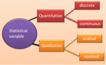
Figure 1. Types of statistics variables.
Descriptive statistics includes two types of variables, namely quantitative variables and qualitative variables.
It can be quantitative if its various modalities are capable of being measured. Or it can be qualitative if its various modalities are not measurable.
It should be noted that only one modality is applied to an individual.
For example: the sex character has two modalities, which are male and female. An individual cannot possess both modalities at the same time.
1.5.1. The Quantitative Variable
It has measurable categories. It is either discrete or continuous.
A quantitative variable is discrete when all of its categories are countable.
For example: the men of the village of KASKALONDAL, banks domiciled in the DRC, etc.
A variable is continuous if its entire range of values is uncountable, meaning that the variable can take any numerical value within a given interval.
1.5.2. The Qualitative Variable
It has non-measurable modalities.
It is either ordinal or nominal.
A qualitative variable is ordinal if its modalities are naturally ordered, arranged.
Example: the size of a company is small, medium, large, etc.
It is qualitative and nominal when its modalities do not admit of order, for example, gender, etc.
1.6. Absolute and Relative Frequency
1.6.1. Absolute Frequency
Is the absolute number of individuals that corresponds to a modality of the statistical variable studied.
The absolute frequency of a modality i of the characteristic X with k modalities is the number of elements of the population that possess the modality of this characteristic.
We denote it ni. Thus n1 is the frequency of the first modality, n2 corresponds to the frequency of the second modality, etc.
The sum of the absolute frequency corresponding to all the modalities of the set studied.
It is denoted by N if it is the total size of the population studied, but by n if it is the total size of the selected sample.
Note that: N = n1+n2+n3+n4+n5++nK
N =i=1kni
with N being the population size and
n =n1+n2+n3+n4+n5++nK
n = i=1kni with n being the sample size
1.6.2. The Relative Frequency
The relative frequency of a modality is a ratio of the corresponding effective of occurrences to the total effective of occurrences.
We note it fi where fi= niN or fi= niN x 100 If frequencies are expressed as a percentage, we also speak of a relative percentage.
The practical case below illustrates the concept of relative frequency:
1.6.3. Illustration
AL BANK is a commercial company with 300 employees, including 198 singles, 94 married, 5 widowers, and 3 divorced.
N is the total number of 300 individuals, that is
n1=198,n2=94, n3=5,n4=3
N = n1+n2+n3+n4
300 = 198+94+5+3
We know that
fi=niNhence, f1=n1N=198300=0,66f2=n1N=94300=0,31333333
f3=n3N=5300=0,01666667f4=n1N=3300=0,01
Fi=f1+f2+f3+f4
=0,66 + 0,31333333 +0,01666667+0,01
=1
OU fi=niN x 100 d’où, f1=n1N*100=198300*100=66%f2=n1N*100=94300*100=31%
f3=n3N*100=5300*100=2%f4=n1N*100=3300*100=1%
F in%=66% + 31%+ 2%+ 1%
=100%
This could be presented in the form of a table and in graphical form, which refers us to chapter 2 of our book.
For the moment, these calculations can easily be performed using the software mentioned above:
2. Relative Frequency Calculations Using EXCEL, EVIEWS and R STUDIO Software
2.1. Relative Frequency Calculations Using EXCEL
Start by opening Excel and then create a variable (a vector) X following:
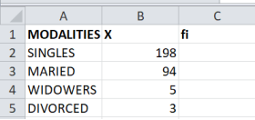
Figure 2. Modalities data.
In B6 write “= somme (B2: B5) “ then “ Enter “ The result appears as follows:
“ 300” but if your computer language is english “somme” is named by “sum”.
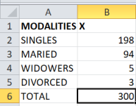
Figure 3. Modalities sum.
Based on the formula for fi studied above, enter the following formula in cell C2
= B2/$B$6 “ then “ Enter “ Once the formula is applied to “C2”, position the mouse cursor there, drag down while holding down the left mouse button. Once the cursor has the shape of a small cross, the calculations will be performed automatically, resulting in the following:
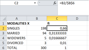
Figure 4. Relative frequency calculations.
To obtain the Fi as a percentage, simply select the relevant column C and then click on% in the formula bar as follows:
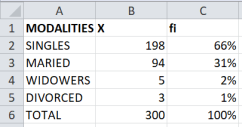
Figure 5. Using EXCEL% to relative frequency calculations.
We get this:
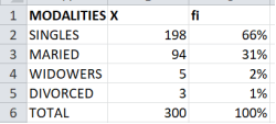
Figure 6. Relative frequency in percentage (%).
Simple Interpretation
66% of AL BANK employees are single, 31% are married, 2% are widowed and 1% is divorced.
Indeed, there’s no single way to interpret a table of statistical results; several methods exist. The goal here is to help you stand out in your field by using refined scientific language. So, instead of saying “AL BANK has many single people and many married people,” say “66% of AL BANK employees are single and 31% are married.” This provides clarity and precision.
2.2. Relative Frequency Calculations with EVIEWS 10
Let’s start by creating a variable X of the 300 individuals composed of the 4 observations:
Open EVIEWS,
In the command bar: enter “create” then “Enter”. A window will open where you specify the data type and then the number of observations or categories. After that, click “OK” as shown in the windows below:
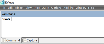
Figure 7. EVIEWS Command bar.
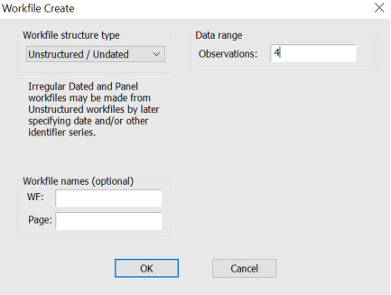
Figure 8. EVIEWS Workfile.
We are now at the next stage:
In the command bar, enter the command “data x” and press “Enter”; your workspace (workfile) is now created.
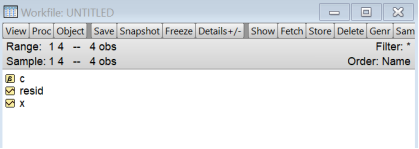
Figure 9. Workfile creation.
Click on the small envelope X and a window will open:
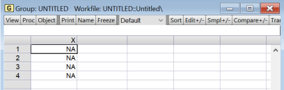
Figure 10. Data workfile.
Replace the NA values with the X values by entering them one after the other or by copying them into Excel using the command “ctrl c” and “ctrl v”.
We obtain this:
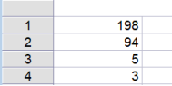
Figure 11. Data Entered.
To find the total, go to the command bar, type the command “stats x”, and press “Enter”. The following statistics will then be displayed:
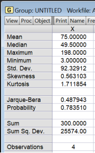
Figure 12. EVIEWS output Statistics.
“Sum” is obviously the sum or total we need. “Observations” are our observations or modalities.
Next, generate a new variable “Fi” using the following commands:
genr Fi = x/ 300” If we want Fi to be expressed as a percentage, we simply need to introduce the multiplication by 100 into the formula for Fi as follows:
genr Fi = x/ 300*100 “.
We arrive at the relative frequency as shown in the table below.
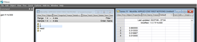
Figure 13. Relative Frequency using Genr command.
2.3. Calculating Relative Frequency with R STUDIO
We open R STUDIO and we create an object or vector X with our 4 values by using the console like this:
X < - (198, 94, 5, 3) “
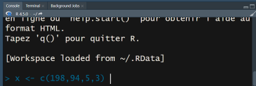
Figure 14. Data Enter using R console.
It should also be deduced that R (or R STUDIO) is very advanced statistical software, it uses a programming language.
The symbol
< -is the assignment operator that allows us to provide values to the object X.
We agree that a set of data of the same nature constitutes a vector for R and is constructed using a function named c. We use it by giving it the list of our data, in parentheses, separated by commas.
For pedagogical reasons, we continue with the same logic as the famous relative frequency (Fi) formula seen previously and submit the following expression to R STUDIO
“ Fi <- X/ 300 “ then “Enter”
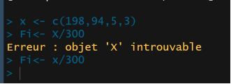
Figure 15. Entered Error in R software.
Remark
Objects in R must always begin with a letter (never a number). R is case-sensitive, meaning that x and X are two different objects.
Therefore, when X is written, R displays “Erreur: objet ‘X’ introuvable” (for “Error: Object ‘X’ not found”).
It is worth remembering that for this software, as with some other programming software, it is essential to be attentive and precise in order to use it correctly.
To see our results for x and Fi, simply type your vector x in the console, then press Enter, then Fi, and press Enter again. We get the following results respectively:
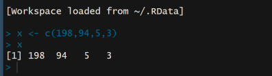
Figure 16. Correct Entered data in R Software.
And
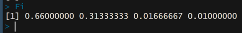
Figure 17. Relative frequency.
To obtain the previous result as a percentage, simply multiply Fi by 100, i.e., write the following in the console:
“Fi*100” then “Enter” This refers to the following output
However, it should be noted that the specifics of frequency calculations under our three software programs will be developed in chapters 1 and 2 of our book.
Figure 18. Relative Frequency in percentage.
Practical case
As an illustration, a very simple example will allow us to see more clearly and to immediately understand the mechanics that we will have to apply and adapt to the specific data.
Sixteen Congolese entrepreneurs are participating in an entrepreneurial training program related to a project funded by a local NGO. Project leaders want to learn more about these entrepreneurs: their age, their business activities, and their marital status.
They are asked to answer a few questions.
It is considered that funding for these entrepreneurs will be likely if a good description of the group is available beforehand.
To achieve this, we first consulted the answer sheets completed by each entrepreneur in need of financing . We then compiled the list reproduced below.
Table 1. Responses from entrepreneurs.

Entrepreneur

How old are you?

At what rhythm are you opening your business?

Do you live alone or with your partner?

1

19

often

alone

2

20

never

partner

3

25

sometimes

partner

4

18

never

alone

5

18

rarely

alone

6

35

sometimes

partner

7

50

rarely

partner

8

37

sometimes

alone

9

60

often

partner

10

42

often

partner

11

34

rarely

alone

12

56

sometimes

partner

13

33

often

alone

14

79

often

partner

15

40

rarely

alone

16

45

often

partner

Here we have three variables: age, which is a quantitative variable, while business opening is an ordinal qualitative variable, and then marital status, which is a nominal qualitative variable.
How can we produce a table of relative frequencies from this data?
We can proceed step by step
step 1. The first step is to establish the absolute frequency for each variable. We can work with the variable “business opening”.
It is agreed that the variable “business opening” has four values, which are initially recorded. Subsequently, the observations are meticulously condensed, taking into account the responses given to this question. The sum of the frequencies corresponds, of course, to the total population or to the relevant sample. We can therefore construct the frequency table as follows:
Table 2. Absolute Frequency Table.

At what rhythm are you opening your business?

Absolute Frequency

often

6

sometimes

4

rarely

4

never

2

Total

16

Let’s move on to the second step, which aims to establish what is called the Cumulative Absolute Frequency.
The operation consists of summing the absolute frequency of the value in question and all the absolute frequencies of the values that precede it.
Table 3. Cumulative Absolute Frequency.

At what rhythm are you opening your business?

Absolute Frequency

Cumulative Absolute Frequency

Often

6

6

Sometimes

4

10

rarely

4

14

never

2

16

Total

16

The cumulative frequency of the last value must equal the total number of cases. For example, from Table 3, we can deduce that 10 individuals say they sometimes or often open their businesses. This type of information lends itself well to cumulative frequency analysis.
The third step consists of transforming the absolute frequency into a relative frequency (proportion or percentage).
Here, each result is reported in relation to the total number of individuals in the series studied: Here, 6 out of 16 often open their businesses, which are 0.375%, resulting in 37.5% as shown below.
Table 4. Relative frequency.

At what rhythm are you opening your business?

Absolute Frequency

Cumulative Absolute Frequency

Relative Frequency (%)

often

6

6

37,5

sometimes

4

10

25

rarely

4

14

25

never

2

16

12,5

Total

16

100

With our three software programs, these calculations take place in a few seconds and this will be covered in the next chapter, because here we have only skipped ahead in order to facilitate understanding for those who will not have the chance to read the pages of other chapters.
Before moving on to the second chapter, it is essential to recall the concept of “class” in statistics.
3. Class and Limit
What is a class in statistics?
A class is a group of values of the variable. It takes the form of an interval closed on the left and open on the right, i.e.
: [a, b]
1) With “a” the inferior limit (or lower limit)
2) “b” the superior limit (or upper limit)
3) « b-a » the amplitude of the class
4) « (b+a) 2 » The center of the class
To construct these intervals, a few rules can be applied
1) If possible, the classes should have the same amplitude
2) The number of classes for a sample of size n can be determined by applying, for example, YULE’s Rule, according to which:
Number of classes =2, 5 n4
The interval between each class is then obtained using the following ratio:
Ymax-YminNumber of classes
With Ymax and Ymin respectively the largest and smallest value of Y in the statistical series.
We agree that Chapter 2 will best address the concepts of “frequencies” and “class”.
Abbreviations

Fi

Relative Frequency

i

Modality of Character

n

Individual Size

N

Population Size

ni

Absolute Frequency or Effective of i Modality


Sigma Is a Greek Letter, It Is Used to Indicate Summation of Elements Like Sample, Population, etc.

Author Contributions
Alain Mbayo Yamwembo: Writing – review & editing
Conflicts of Interest
The author declares no conflict of interest.
References
[1] MBAYO YAMWEMBO, A. Applied statistics of Business: Analysis of practical cases using EVIEWS and SPSS. working paper. prosinec 2025.
[2] ANDERSON, D. R., SWEENEY, D. J., WILLIAMS, T. A. Statistics for Business and Economics. 11. ed. Mason, Ohio: South-Western, 2011.
[3] DE SÈDE-MARCEAU, M.-H. introduction to the descriptive statistics [online]. course notes. 2010. Dostupné z: chrome-extension:
[4] MASAMBA FAMODE, D. Elements of descriptive statistics. la tourbière. 2023.
[5] MONTGOMERY, D. C., RUNGER, G. C. Applied Statistics and Probability for Engineers. Seventh edition. Hoboken, NJ: Wiley, 2018. EMEA edition.
[6] MIAH, A. Q. Applied Statistics for Social and Management Sciences [online]. 1st ed. 2016. Singapore: Springer, 2016. SpringerLink Bücher. Dostupné z:
[7] A. SHAYIB, M. Applied Statistics [online]. 1 st. Ethiopia: bookboon, 2013. Dostupné z: chrome-extension:
[8] ANDERSON, D. R., SWEENEY, D. J. (eds.). Statistics for Business and Economics 12e. 12. ed. Mason, Ohio: South-Western, Cengage Learning, 2014.
[9] MCCLAVE, J. T., BENSON, P. G., SINCICH, T. Statistics for Business and Economics. 14 edition, global edition. Harlow, England: Pearson, 2022.
[10] TERRAZA, V., TOQUE, C. Statistical analysis for banking and financial management: applications with R. Bruxelles: Of superior Boeck, 2013. Economic openings.
Cite This Article
  • APA Style

    Yamwembo, A. M. (2026). The First Notions of Descriptive Statistics Applications with EXCEL, EVIEWS and R STUDIO. American Journal of Applied Mathematics, 14(3), 129-138. https://doi.org/10.11648/j.ajam.20261403.13

    Copy | Download

    ACS Style

    Yamwembo, A. M. The First Notions of Descriptive Statistics Applications with EXCEL, EVIEWS and R STUDIO. Am. J. Appl. Math. 2026, 14(3), 129-138. doi: 10.11648/j.ajam.20261403.13

    Copy | Download

    AMA Style

    Yamwembo AM. The First Notions of Descriptive Statistics Applications with EXCEL, EVIEWS and R STUDIO. Am J Appl Math. 2026;14(3):129-138. doi: 10.11648/j.ajam.20261403.13

    Copy | Download

  • @article{10.11648/j.ajam.20261403.13,
      author = {Alain Mbayo Yamwembo},
      title = {The First Notions of Descriptive Statistics Applications with EXCEL, EVIEWS and R STUDIO},
      journal = {American Journal of Applied Mathematics},
      volume = {14},
      number = {3},
      pages = {129-138},
      doi = {10.11648/j.ajam.20261403.13},
      url = {https://doi.org/10.11648/j.ajam.20261403.13},
      eprint = {https://article.sciencepublishinggroup.com/pdf/10.11648.j.ajam.20261403.13},
      abstract = {This paper defines and explains, in simple and clear terms, key concepts of descriptive statistics and connects statistical theory with applied statistical practice through real cases. It begins by clarifying the meaning of statistics and the basic notions used daily in many fields, while distinguishing statistics as a science and an art from statistics understood as data and measures. The study adopts the following definition: “Statistics is simply an art and a science that allows for the collection, analysis, presentation, and interpretation of data for the purpose of making decisions about any phenomenon under study.” To illustrate these concepts, practical applications were carried out using real data from two institutions: AL BANK and a non-governmental organization. For the calculations and applications, EXCEL, EVIEWS, and R STUDIO were used. In the AL BANK case, relative frequencies were calculated step by step with the three software programs and then verified manually using the mathematical frequency formula. In Excel, the process involved entering the data, computing the total number of observations, and calculating the relative frequencies. In EVIEWS, the observations were entered, descriptive statistical measures including the total were obtained, and relative frequencies were then calculated. In R STUDIO, the data were entered as a vector and relative frequencies were computed. The three methods produced identical results, showing that 66% of AL BANK employees are single, 31% are married, 2% are widowed, and 1% is divorced. In the non-governmental organization case, the variable “business opening” was used to calculate cumulative frequencies. The procedure consisted of constructing the absolute frequency table, the relative frequency table, and then the cumulative absolute and cumulative relative frequency tables. The analysis showed that, in terms of cumulative absolute frequency, ten individuals reported that they sometimes or often open their businesses. Regarding relative frequencies, six out of sixteen individuals reported often opening their businesses (37.5%), while 25% sometimes open their businesses, 25% rarely open them, and 12.5% never open them. These findings highlight the importance of frequency as the one of the fundamental concepts of applied statistics.},
     year = {2026}
    }
    

    Copy | Download

  • TY  - JOUR
    T1  - The First Notions of Descriptive Statistics Applications with EXCEL, EVIEWS and R STUDIO
    AU  - Alain Mbayo Yamwembo
    Y1  - 2026/05/21
    PY  - 2026
    N1  - https://doi.org/10.11648/j.ajam.20261403.13
    DO  - 10.11648/j.ajam.20261403.13
    T2  - American Journal of Applied Mathematics
    JF  - American Journal of Applied Mathematics
    JO  - American Journal of Applied Mathematics
    SP  - 129
    EP  - 138
    PB  - Science Publishing Group
    SN  - 2330-006X
    UR  - https://doi.org/10.11648/j.ajam.20261403.13
    AB  - This paper defines and explains, in simple and clear terms, key concepts of descriptive statistics and connects statistical theory with applied statistical practice through real cases. It begins by clarifying the meaning of statistics and the basic notions used daily in many fields, while distinguishing statistics as a science and an art from statistics understood as data and measures. The study adopts the following definition: “Statistics is simply an art and a science that allows for the collection, analysis, presentation, and interpretation of data for the purpose of making decisions about any phenomenon under study.” To illustrate these concepts, practical applications were carried out using real data from two institutions: AL BANK and a non-governmental organization. For the calculations and applications, EXCEL, EVIEWS, and R STUDIO were used. In the AL BANK case, relative frequencies were calculated step by step with the three software programs and then verified manually using the mathematical frequency formula. In Excel, the process involved entering the data, computing the total number of observations, and calculating the relative frequencies. In EVIEWS, the observations were entered, descriptive statistical measures including the total were obtained, and relative frequencies were then calculated. In R STUDIO, the data were entered as a vector and relative frequencies were computed. The three methods produced identical results, showing that 66% of AL BANK employees are single, 31% are married, 2% are widowed, and 1% is divorced. In the non-governmental organization case, the variable “business opening” was used to calculate cumulative frequencies. The procedure consisted of constructing the absolute frequency table, the relative frequency table, and then the cumulative absolute and cumulative relative frequency tables. The analysis showed that, in terms of cumulative absolute frequency, ten individuals reported that they sometimes or often open their businesses. Regarding relative frequencies, six out of sixteen individuals reported often opening their businesses (37.5%), while 25% sometimes open their businesses, 25% rarely open them, and 12.5% never open them. These findings highlight the importance of frequency as the one of the fundamental concepts of applied statistics.
    VL  - 14
    IS  - 3
    ER  - 

    Copy | Download

Author Information
  • Abstract
  • Keywords
  • Document Sections

    1. 1. Generalities
    2. 2. Relative Frequency Calculations Using EXCEL, EVIEWS and R STUDIO Software
    3. 3. Class and Limit
    Show Full Outline
  • Abbreviations
  • Author Contributions
  • Conflicts of Interest
  • References
  • Cite This Article
  • Author Information